Vector Field and Flow Visualization
The study and research of fluid behavior and properties have been a challenging topic due to the invisible patterns of fluid (e.g., air, water). Flow visualization is used to make flow patterns visible so that we can visually acquire qualitative and quantitative flow information. A vector field (or flow field) is a mapping F(P)=V that assigns a vector V to each point P in the domain U. In reality, the domain U is a 3D space such as a rectilinear grid, which can be divided into evenly-sized cubes or voxels. The flow within the space can be represented by vectors. A vector (vx, vy, vz) is assigned to each voxel to indicate both direction and magnitude of the flow at the center of that voxel. Vectors that are not at voxel centers are linearly interpolated. In the 2D space, the domain U is represented by a 2D grid, and each cell of this grid is assigned a vector (vx, vy) that indicates both direction and magnitude of the flow at the center of that cell, as shown in the figure below.
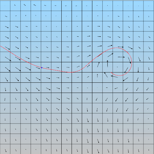
A 2D vector field and a streamline
When all the time derivatives of a flow field vanish, the flow is considered to be a steady flow. In other words, steady flow refers to the condition where the fluid properties at a point in the system do not change over time. When time does affect the behavior of the flow, we consider the flow as an unsteady flow. The most common way to visualize a flow field is to depict the “paths” that fluid elements will follow throughout the time. These paths are called streamlines (for a steady flow field) or pathlines (for an unsteady flow field).
Line Integral Convolution Image
A line integral convolution or (LIC) image uses a dense texture to depict the overview streamline patterns on a 2D flow data set or one slice of a 3D flow data set. It works by adding a random static pattern of black-and-white paint sources to visualize the flow field. As the flow passes by the sources each fluid particle picks up some of the source intensity. The result is a random striped texture where points along the same streamline tends to have similar intensities.
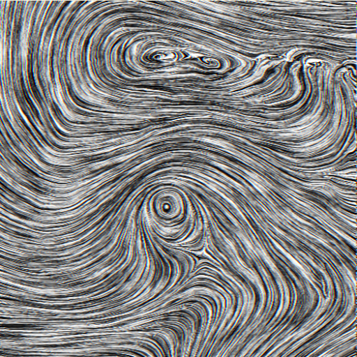
LIC image
Streamlines
A streamline is a curve tangent to the flow field everywhere, as shown in the figure below. The streamlines are drawn in red while the vectors are drawn in blue. Intuitively, a streamline is the path that a massless particle will follow if released in a steady flow field. If a small ball is placed into a water flow, and assuming the water flow does not change over time (i.e., a steady flow), the trajectory of the ball is a streamline.
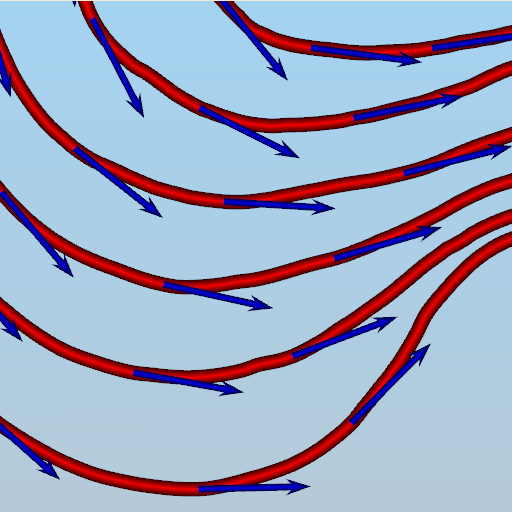
Streamlines
Pathlines
A pathline is the trajectory that an individual fluid particle will follow in an unsteady flow field, as shown in the figure below. The pathlines seeded from a rake are drawn in yellow while the underlying unsteady flow field is depicted using LIC textures. The concept of pathline is similar to that of streamline except that the underlying flow field is unsteady. Intuitively, if a small ball is placed into a water flow, and the water flow changes over time (i.e., an unsteady flow), the ball will follow the flow direction at each time step. In this case, the trajectory of the ball is a pathline.
Pathlines
Streaklines
A streakline is the locus of points of all the fluid particles that have passed continuously through a particular spatial point in the past. Intuitively, if we place multiple small balls into the water flow at the same position but at different time steps, the streakline is the path by connecting all the balls in the placement order. Another real-world example of streaklines is smoke, where all particles are released at the same position, but at different time steps. As shown in the figure below, streaklines are closely related to pathlines. In the figure, the pathlines are drawn in yellow while the streakline is drawn in green. Given a set of pathlines traced from the same position at different time steps, connecting all points at the same time step forms a streakline.
Streaklines
Timelines
A timeline is a line formed by a set of fluid particles that were marked at a previous instant in time, creating a curve that is displaced over time as the particles move. Intuitively, imagine that we place several small balls into a water flow, and allow the balls to follow the flow. At a certain time step, the path that connects all the balls is a timeline. As shown in the figure below, timelines are closely related to pathlines. In the figure, the pathlines are drawn in yellow while the timeline is drawn in purple. Given a set of pathlines traced from the same time step at different positions, connecting all the points at the same time step forms a timeline.
Timelines
Critical Points
A critical point is a position in a flow field domain where the velocity vanishes. For a 2D flow field, there are six types of critical points: saddle points, repelling nodes, attracting nodes, centers, repelling focuses, and attracting focuses. The following figures illustrate the flow pattern around each of these six critical points.
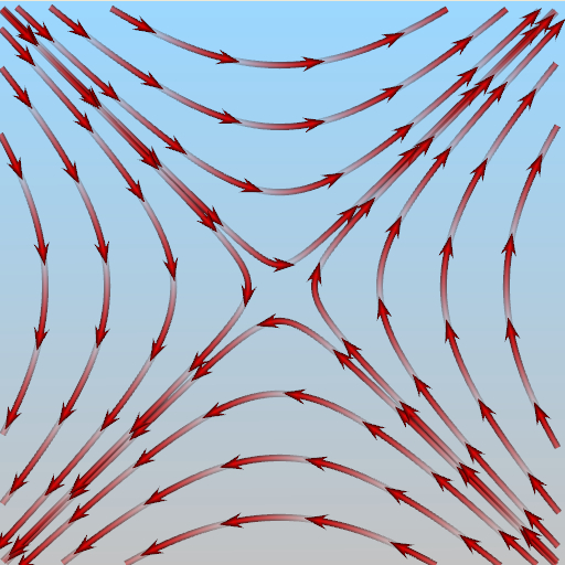 Saddle |
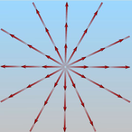 Repelling Node |
 Attracting Node |
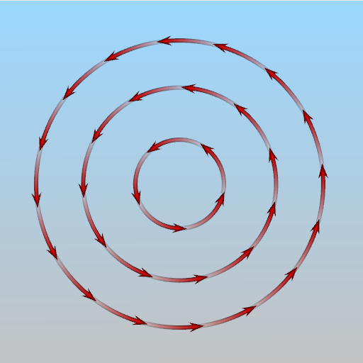 Center |
 Repelling Focus |
 Attracting Focus |
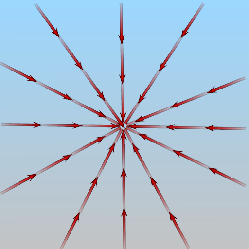
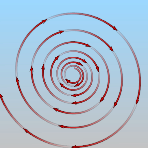
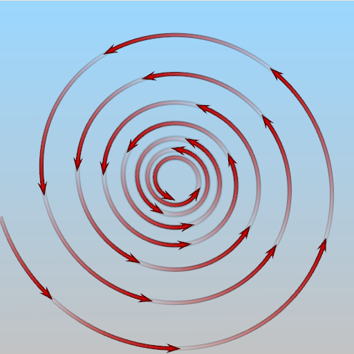
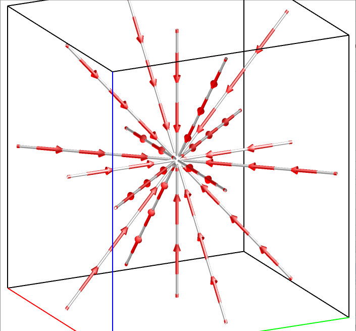
For a 3D flow field, there are five types of critical points: spiral, spiral saddle, saddle, source, and sink. The following figures illustrate the flow pattern around each type of these five critical points.
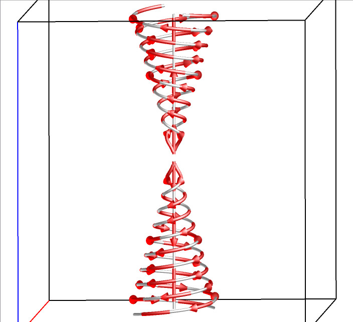 Spiral F(x,y,z)=(y-x,-x-y,-z) |
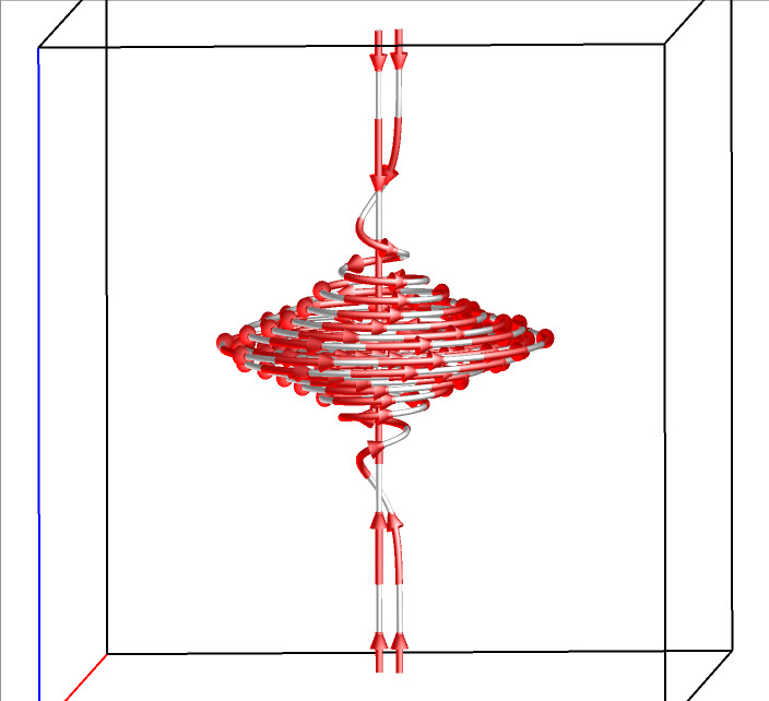 Spiral Saddle F(x,y,z)=(y-x,-x-y,z) |
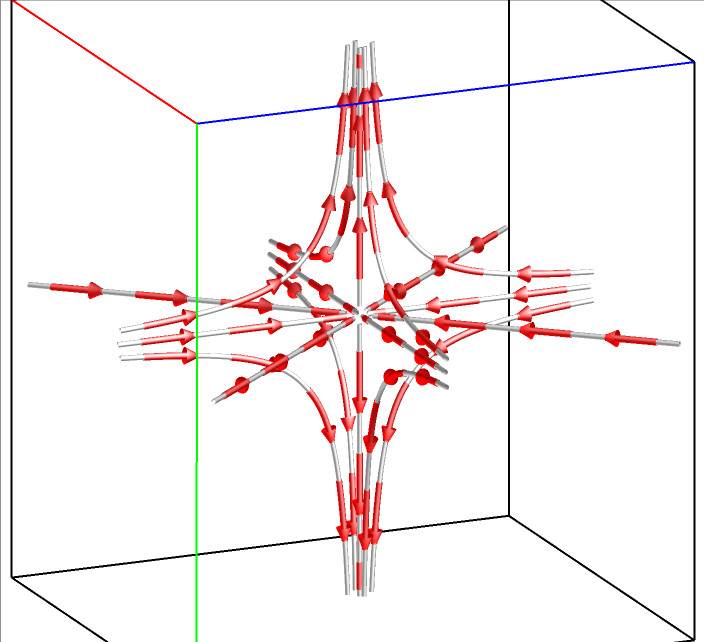 Saddle F(x,y,z)=(-x,-y,z) |
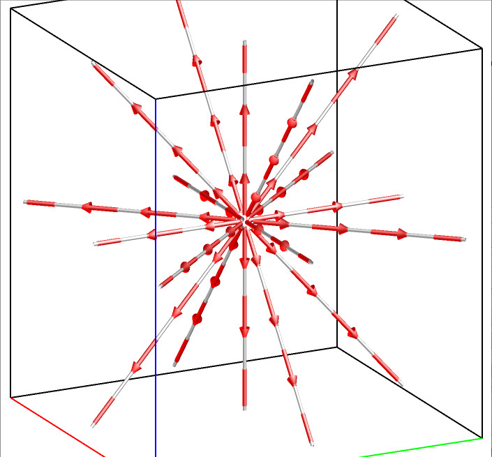 Source F(x,y,z)=(x,y,z) |
 Sink F(x,y,z)=(-x,-y,-z) |
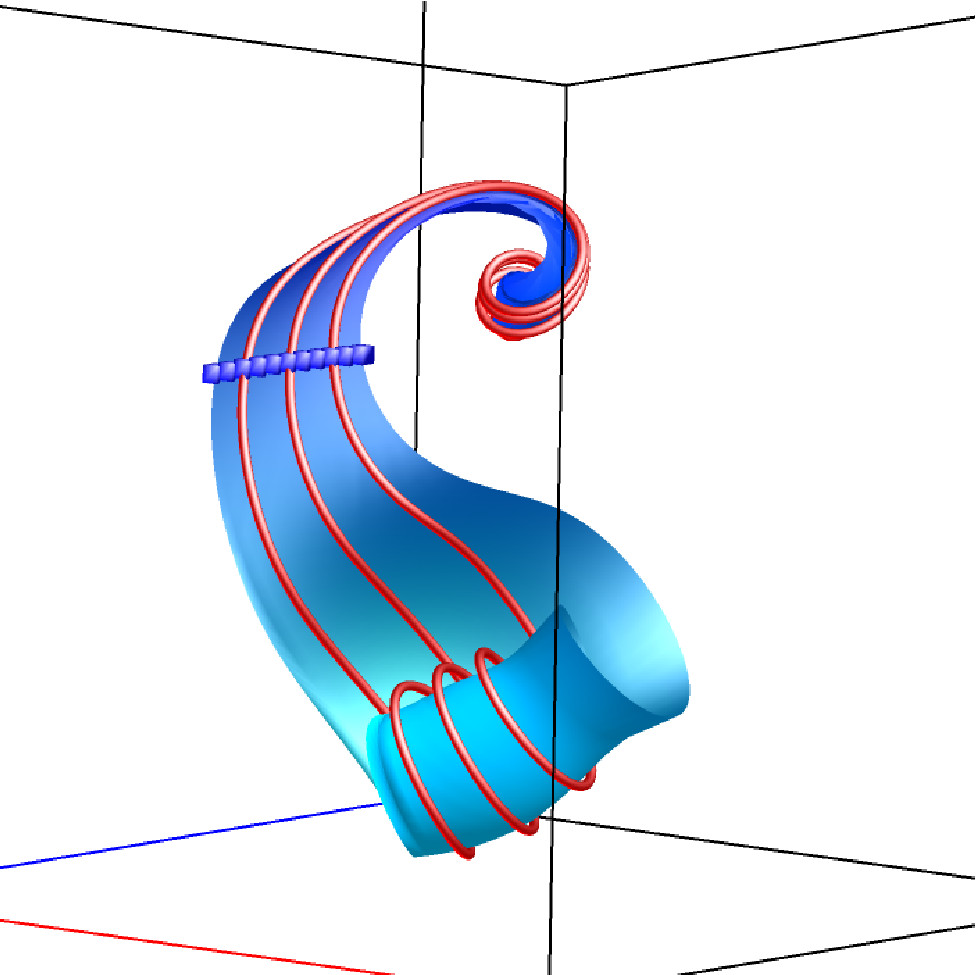
Stream Surface
A stream surface is a continuous surface that is everywhere tangent to the vector it passes, which can be obtained from streamlines traced from a densely seeded curve.
The images below show multiple surface overview and single surface inspection with streamlines and streamline animation. The multiple surface overview provides an overall impression of the flow field by displaying multiple stream surfaces at the same time. The single surface inspection allows one surface to be examined along with streamlines and streamline animation, without occlusion from other surfaces.
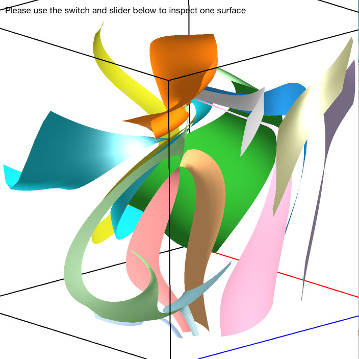 Multiple surfaces with unique color for each surface |
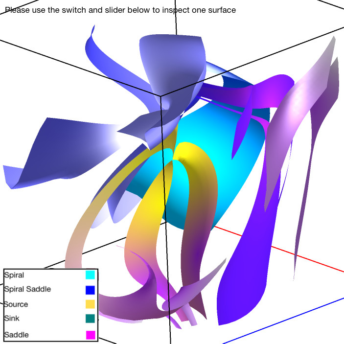 Multiple surfaces with colors by the types of related critical points |
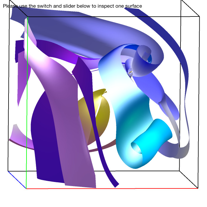 Multiple surfaces from another viewpoint |
 Single surface + streamlines |
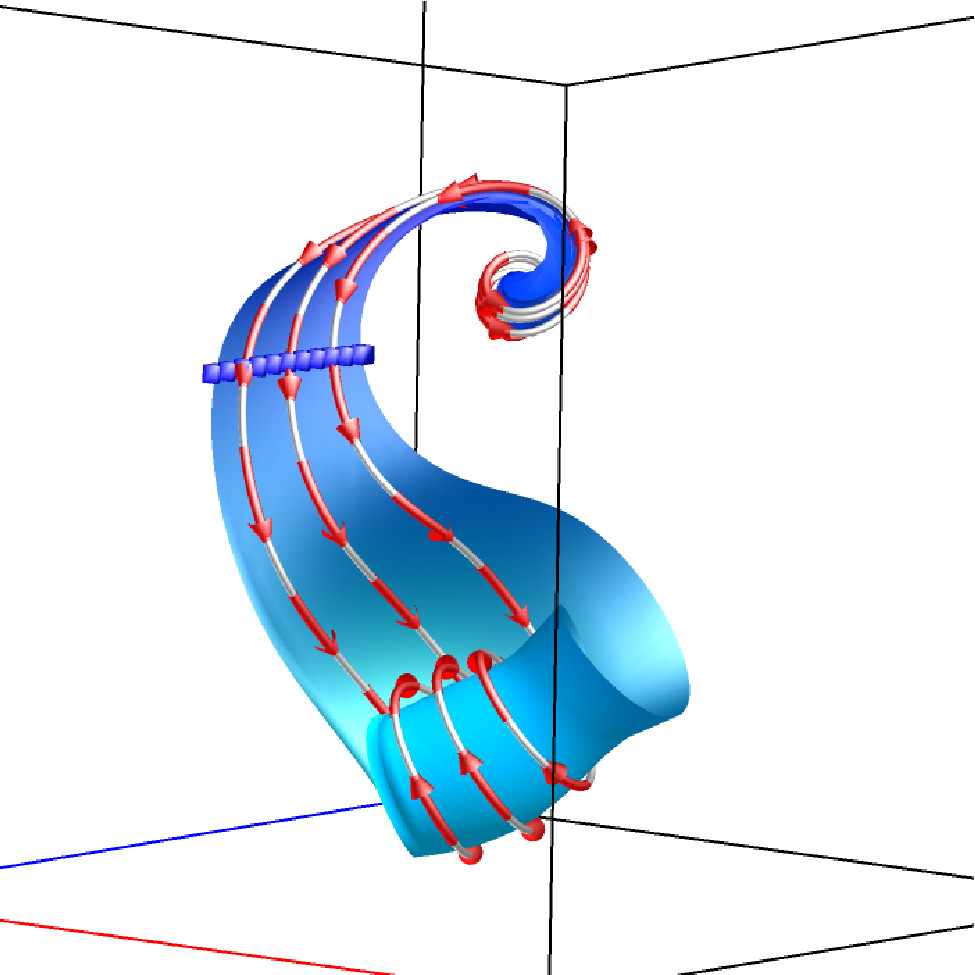 Single surface + streamline animation |
Download
FlowVisual for 2D Flow Field Visualization
- Click here to download the Windows version: 2dflowvis-win.zip
- Unzip the files into a directory 2dflowvis
- Double-click 2dflowvis.exe in the directory to run the program
- If the program cannot start on a windows 64-bit machine, please follow these instructions to run the program in compatibility mode:
- Right click on the executable (2dflowvis.exe) and select “Properties”.
- Select “Compatibility” tab from the pop-up window.
- Check “Run this program in compatibility mode for:” and select “Windows XP (Service Pack 2)” from the combo box.
- Apply the changes by clicking “OK” or “Apply”.
- Click here to download the 32-bit Linux version: 2dflowvis-linux32.tar.gz
or here to download the 64-bit Linux version: 2dflowvis-linux64.tar.gz- In a terminal, untar the files using the following command
tar -xzvf 2dflowvis-linux32.tar.gz
or
tar -xzvf 2dflowvis-linux64.tar.gz
- Change the current directory to 2dflowvis
- In the same terminal, run the program using the following command
./2dflowvis
- In a terminal, untar the files using the following command
- Click here to download the Mac version (OS X Sierra): 2dflowvis-mac.tar.gz
- Double-click 2dflowvis-mac.tar.gz to untar the program
- Double-click 2dflowvis-mac to run the program
FlowVisual for 3D Flow Field Visualization
- The tool is developed for iPad and currently available at the App Store as FlowVisual.
Publications
Man Wang, Jun Tao, Jun Ma, Yang Shen, and Chaoli Wang. FlowVisual: A Visualization App for Teaching and Understanding 3D Flow Field Concepts. In Proceedings of IS&T Conference on Visualization and Data Analysis, San Francisco, CA, pages 476-1-476-10, Feb 2016.
Man Wang, Jun Tao, Chaoli Wang, Ching-Kuang Shene, and Seung Hyun Kim. FlowVisual: Design and Evaluation of a Visualization Tool for Teaching 2D Flow Field Concepts. In Proceedings of American Society for Engineering Education Annual Conference, Atlanta, GA, pages 23.609.1-23.609-20, Jun 2013.
Data Set
The flow data used in this tutorial include a hurricane simulation data set and a synthesized five critical points data set. The hurricane simulation data set is made available through IEEE Visualization 2004 Contest. The five critical points data set is made available by Dr. Alex Pang via his IEEE Visualization 2005 paper Strategy for Seeding 3D Streamlines.
Contact