Post by Michael Dietze and Ann Raiho
What is state data assimilation (SDA)?
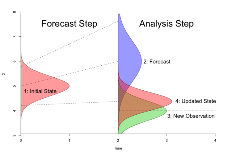
SDA is the process of using observed data to update the internal STATE estimates of a model, as opposed to using data for validation or parameter calibration. The exact statistical methods vary, but generally this involves running models forward, stopping at times where data were observed, nudging the model back on track, and then restarting the model run (Figure 1). The approached being employed by the modeling teams in PalEON are all variations of ENSEMBLE based assimilation, meaning that in order to capture the uncertainty and variability in model predictions, during the analysis step (i.e. nudge) we update both the mean and the spread of the ensemble based on the uncertainties in both the model and the data. Importantly, we don’t just update the states that we observed, but we also update the other states in the model based on their covariances with the states that we do observe. For example, if we update composition based on pollen or NPP based on tree rings, we also update the carbon pools and land surface fluxes that co-vary with these.

Figure 1. Schematic of how state data assimilation works. From an initial state (shown as pink in the Forecast Step) you make a prediction (blue curve in the Analysis step). Then compare your data or new observation (green in the Analysis step) to the model prediction (blue) and calculate an updated state (pink in the Analysis step).
There are many components in the PalEON SDA and many people are involved. In all methods being employed by PalEON modeling teams, the uncertainty in the meteorological drivers is a major component of the model ensemble spread. Christy Rollinson has developed a workflow that generates an ensemble of ensembles of meteorological drivers – first she starts with an ensemble of different GCM’s that have completed the ‘last millennia’ run (850-1850 AD) and then downscales each GCM in space and time, generating an ensemble of different meteorological realizations for each GCM that propagates the downscaling uncertainty. John Tipton and Mevin Hooten then update this ensemble of ensembles, providing weights to each based on their fidelity with different paleoclimate proxies over different timescales. In addition to the meteorological realizations, some of the techniques being employed also accommodate model parameter error and model process error (which is like a ‘residual’ error after accounting for observation error in the data).
Why are we doing SDA in PalEON?
In the PalEON proposals we laid out four high-level PalEON objectives: Validation, Inference, Initialization, and Improvement. Our previous MIP (Model Intercomparison Project) activities at the site and regional scale were focuses specifically on the first of these, Validation. By contrast, SDA directly informs the next two (Inference, Initialization). Both the SDA and the MIP indirectly support the fourth (Improvement).
In terms of Inference, the central idea here is to formally fuse models and data to improve our ability to infer the structure, composition, and function of ecosystems on millennial timescales. Specifically, by leveraging the covariances between observed and unobserved states we’re hoping that models will help us better estimate what pre- and early-settlement were like, in particular for variables not directly related to our traditional paleo proxies (e.g. carbon pools, GPP, NEE, water fluxes, albedo). The last millennium is a particularly important period to infer as it’s the baseline against which we judge anthropogenic impacts, but we lack measurements for many key variables for that baseline period. We want to know how much we can reduce the uncertainty about that baseline.
In terms of Initialization, a key assumption in many modeling exercises (including all CMIP / IPCC projections) is that we can spin ecosystems up to a presettlement ‘steady state’ condition. Indeed, it is this assumption that’s responsible for there being far less model spread at 1850 than for the modern period, despite having far greater observations for the modern. However, no paleoecologist believes the world was at equilibrium prior to 1850. Our key question is “how much does that assumption matter?” Here we’re using data assimilation to force models to follow the non-equilibrium trajectories they actually followed and assessing how much impact that has on contemporary predictions.
Finally, SDA gives us a new perspective on model validation and improvement. In our initial validation activity, as well as all other MIPs and most other validation activities, if a model gets off to a wrong start, it will generally continue to perform poorly thereafter even if it correctly captures processes responsible for further change over time. Here, by continually putting the model back ‘on track’ we can better assess the ability of models to capture the system dynamics over specific, fixed time steps and when in time & space it makes reasonable vs unreasonable predictions.
SDA Example
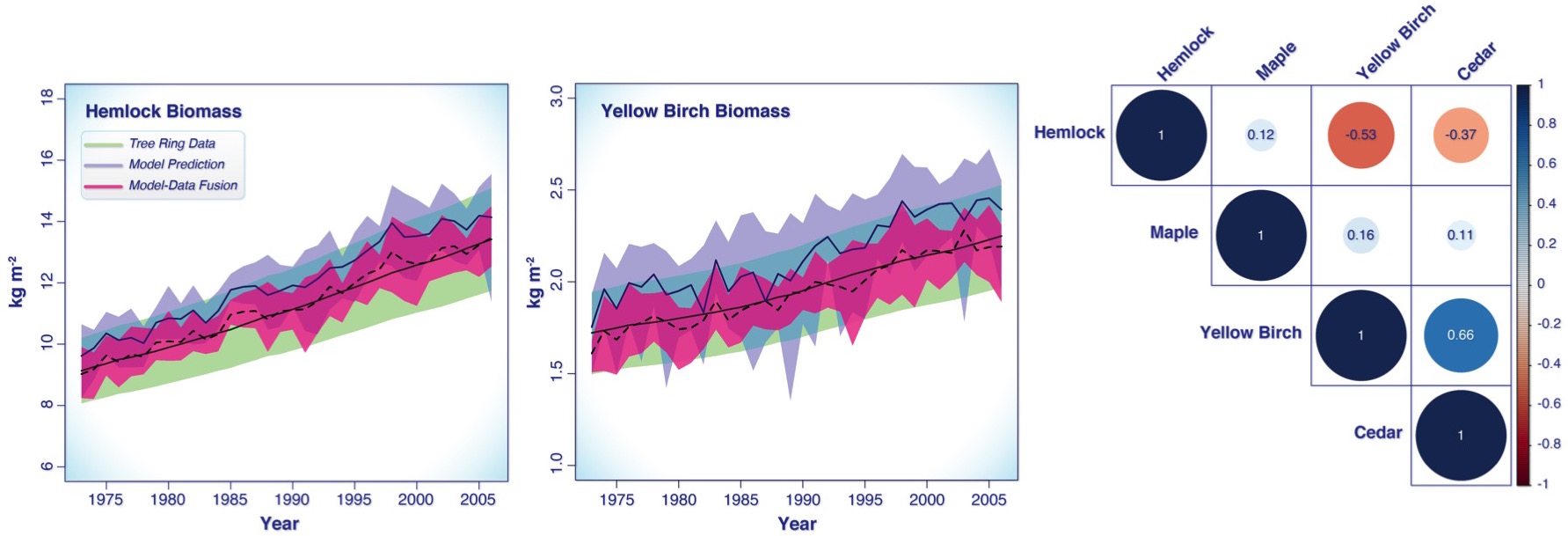
Figure 2 shows a PalEON SDA example for a 30 year time period using tree ring estimates of aboveground biomass for four tree species from data collected at UNDERC and a forest gap model called LINKAGES. The two plots show the tree ring data for hemlock and yellow birch in green, the model prediction in purple and the pink is how the data “nudge” the model. The correlation plot on the right represents the process error correlation matrix. That is, it shows what correlations are either missing in LINKAGES or are over represented. For example, the negative correlations between hemlock vs. yellow birch and cedar suggest there’s a negative interaction between these species that is stronger than LINKAGES predicted, while at the same time yellow birch and cedar positively covary more than LINKAGES predicted. One interpretation of this is that hemlock is a better competitor in this stand, and yellow birch and cedar worse, than LINKAGES would have predicted. Similarly, the weak correlations of all other species with maple doesn’t imply that maples are not competing, but that the assumptions built into LINKAGES are already able to capture the interaction of this species with its neighbors.

Figure 2. SDA example of aboveground biomass in the LINKAGES gap model. The left and middle plots are the biomass values through time given the data (green), the model predictions (purple), and the updated model-data output (pink). The plot on the right is a correlation plot representing the process error correlation matrix.
