State Data Assimilation and PalEON

Post by Michael Dietze and Ann Raiho

What is state data assimilation (SDA)?

SDA is the process of using observed data to update the internal STATE estimates of a model, as opposed to using data for validation or parameter calibration. The exact statistical methods vary, but generally this involves running models forward, stopping at times where data were observed, nudging the model back on track, and then restarting the model run (Figure 1). The approached being employed by the modeling teams in PalEON are all variations of ENSEMBLE based assimilation, meaning that in order to capture the uncertainty and variability in model predictions, during the analysis step (i.e. nudge) we update both the mean and the spread of the ensemble based on the uncertainties in both the model and the data. Importantly, we don’t just update the states that we observed, but we also update the other states in the model based on their covariances with the states that we do observe. For example, if we update composition based on pollen or NPP based on tree rings, we also update the carbon pools and land surface fluxes that co-vary with these.

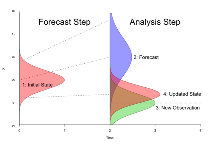
Figure 1. Schematic of how state data assimilation works. From an initial state (shown as pink in the Forecast Step) you make a prediction (blue curve in the Analysis step). Then compare your data or new observation (green in the Analysis step) to the model prediction (blue) and calculate an updated state (pink in the Analysis step).

There are many components in the PalEON SDA and many people are involved. In all methods being employed by PalEON modeling teams, the uncertainty in the meteorological drivers is a major component of the model ensemble spread. Christy Rollinson has developed a workflow that generates an ensemble of ensembles of meteorological drivers – first she starts with an ensemble of different GCM’s that have completed the ‘last millennia’ run (850-1850 AD) and then downscales each GCM in space and time, generating an ensemble of different meteorological realizations for each GCM that propagates the downscaling uncertainty. John Tipton and Mevin Hooten then update this ensemble of ensembles, providing weights to each based on their fidelity with different paleoclimate proxies over different timescales. In addition to the meteorological realizations, some of the techniques being employed also accommodate model parameter error and model process error (which is like a ‘residual’ error after accounting for observation error in the data).

Why are we doing SDA in PalEON?

In the PalEON proposals we laid out four high-level PalEON objectives: Validation, Inference, Initialization, and Improvement. Our previous MIP (Model Intercomparison Project) activities at the site and regional scale were focuses specifically on the first of these, Validation. By contrast, SDA directly informs the next two (Inference, Initialization). Both the SDA and the MIP indirectly support the fourth (Improvement).

In terms of Inference, the central idea here is to formally fuse models and data to improve our ability to infer the structure, composition, and function of ecosystems on millennial timescales. Specifically, by leveraging the covariances between observed and unobserved states we’re hoping that models will help us better estimate what pre- and early-settlement were like, in particular for variables not directly related to our traditional paleo proxies (e.g. carbon pools, GPP, NEE, water fluxes, albedo). The last millennium is a particularly important period to infer as it’s the baseline against which we judge anthropogenic impacts, but we lack measurements for many key variables for that baseline period. We want to know how much we can reduce the uncertainty about that baseline.

In terms of Initialization, a key assumption in many modeling exercises (including all CMIP / IPCC projections) is that we can spin ecosystems up to a presettlement ‘steady state’ condition. Indeed, it is this assumption that’s responsible for there being far less model spread at 1850 than for the modern period, despite having far greater observations for the modern. However, no paleoecologist believes the world was at equilibrium prior to 1850. Our key question is “how much does that assumption matter?” Here we’re using data assimilation to force models to follow the non-equilibrium trajectories they actually followed and assessing how much impact that has on contemporary predictions.

Finally, SDA gives us a new perspective on model validation and improvement. In our initial validation activity, as well as all other MIPs and most other validation activities, if a model gets off to a wrong start, it will generally continue to perform poorly thereafter even if it correctly captures processes responsible for further change over time. Here, by continually putting the model back ‘on track’ we can better assess the ability of models to capture the system dynamics over specific, fixed time steps and when in time & space it makes reasonable vs unreasonable predictions.

SDA Example

Figure 2 shows a PalEON SDA example for a 30 year time period using tree ring estimates of aboveground biomass for four tree species from data collected at UNDERC and a forest gap model called LINKAGES.  The two plots show the tree ring data for hemlock and yellow birch in green, the model prediction in purple and the pink is how the data “nudge” the model. The correlation plot on the right represents the process error correlation matrix.  That is, it shows what correlations are either missing in LINKAGES or are over represented. For example, the negative correlations between hemlock vs. yellow birch and cedar suggest there’s a negative interaction between these species that is stronger than LINKAGES predicted, while at the same time yellow birch and cedar positively covary more than LINKAGES predicted. One interpretation of this is that hemlock is a better competitor in this stand, and yellow birch and cedar worse, than LINKAGES would have predicted. Similarly, the weak correlations of all other species with maple doesn’t imply that maples are not competing, but that the assumptions built into LINKAGES are already able to capture the interaction of this species with its neighbors.

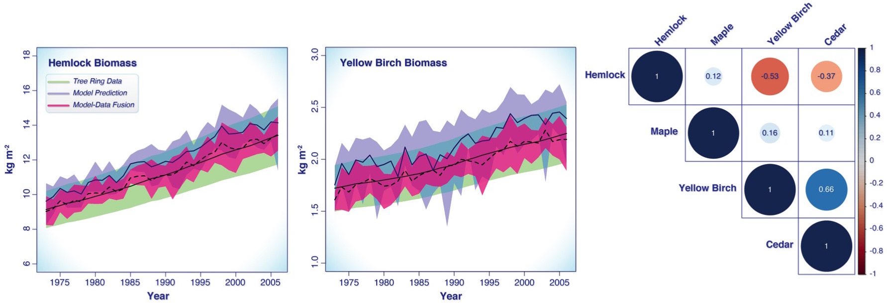
Figure 2. SDA example of aboveground biomass in the LINKAGES gap model. The left and middle plots are the biomass values through time given the data (green), the model predictions (purple), and the updated model-data output (pink). The plot on the right is a correlation plot representing the process error correlation matrix.


Models Part 3: Using Ecosystem Models to Advance Ecology

Post by Christine Rollinson, Post-doc at Boston University working with Michael Dietze.

After a bit of a break and some time back out in the woods, for the PalEON blog and myself, it’s time to wrap up our series of posts on the ecosystem modeling side of PalEON.  In the first post, we talked about why a paleoecological research group is using ecosystem models.  The second post took us behind the curtain and down the rabbit hole to describe a bit of the how of the modeling process.  Now it’s time to take a step back again and talk about what we are learning from the PalEON Model Inter-comparison Project (MIP).

Figure 1

Above is a figure showing aboveground biomass at Harvard Forest from the different PalEON MIP models. The first question most people want know is: Which model is right (or at least closest to reality)?  Well, the fact of the matter is, we don’t really know.  We know that modern biomass at the Harvard Forest is around 100 Mg C per hectare.  Most models are in the right ballpark, but each has a very different path it took to get there.  When we go back in time beyond the past few decades the data available to validate most of these models is extremely sparse.  PalEON has gathered pollen samples at Harvard forest and other MIP sites as well as pre-settlement vegetation records for most of the northeast.  The settlement vegetation records have provided a biomass benchmark for some of our western MIP sites, but aside from that, all other pre-1700 information currently available for comparison with models is based on forest composition.

So how do we evaluate these different models when we don’t actually know what these forests were like 1,000 years ago?  In the absence of empirical benchmarks, we are left comparing the models to each other.  A typical approach would then be to look at each model and try to explain why it has a particular pattern or is different from another model.  For example, why does ED have that giant spike in the 11th century? (We’re still trying to figure that one out; see previous post on debugging.)

Figure 2: The PalEON MIP isn’t the only model comparison project to see models predicting vastly different conditions in time periods that have no data available for comparison. This figure shows similar problems in CMIP51.

Figure 2: The PalEON MIP isn’t the only model comparison project to see models predicting vastly different conditions in time periods that have no data available for comparison. This figure shows similar problems in CMIP51.


The purpose of a multi-model comparison doesn’t necessarily need to be identifying a single “best” or most accurate model.  As an ecologist with PalEON, my goal is to avoid dissecting individual models and instead focus on the big picture and answer questions where output from a single model would be insufficient.

I like to view the PalEON MIP in the same way I would view an empirical-based study that is trying to find cohesive ecological patterns across many field sites or ecosystems.  An incredible about of detailed information can be gleaned from a study based in a single site or region, but these types of studies have their limitations.  Single-site studies have extraordinarily detailed information about plant physiology, ecosystem interactions, and direct effects of warming through experimentation. I think working with a single ecosystem model is very similar to performing a single-site field study.  With one model, you can run simulations to identify potential cause-and-effect relationships, but at the end of the day, the observed response may only be an artifact of that particular model’s structure and not representative of what happens in the real world.

Working with a multi-model comparison is like working with a continental- or global-scale data set.  There’s always a temptation to dig into the story of indvidual sites (or in this case models).  Each site or model has it’s own interesting quirks, stories, and contributions to ecology that a researcher could easily use to build a career (as many have). However, if we think about ideas that have formed the fundamentals of ecology, ideas such as natural selection, carrying capacity, or biogeography, these ideas are those that apply across taxa and ecosystems.  To draw the parallel with modeling, if we want to move away from a piecemeal approach to ecosystem modeling and find synthetic trends, test ecological theories, and identify areas of greatest uncertainty, we need to draw comparisons across many models.  The PalEON MIP, with detailed output from more than 10 models on ecosystem structure and function from millenial-length runs at six sites, is the perfect model data set to look at these sort of questions.

Figure 3

Current PalEON MIP analyses are investigating a wide range of ecological patterns and processes such as the role of temporal scale in understanding causes of ecosystem variation, transitions in vegetation composition, and ecological resilience after extreme events.  With the PalEON MIP, we are first identifying patterns that we know exist in nature such as concurrent shifts in climate and species composition or a given sensitivity of NPP to temperature. We can then find out if and when these patterns occur in the model and only then, look at similarities or differences among the models that might explain patterns of model behavior across models.  Additionally, my personal ecological research interests have led me to use these models to test conceptual ecological theories regarding the role of temporal scale in paleoecological data that have thus far been difficult to assess with empirical data (Fig. 4).

Figure 4

If there’s one point I want you to take away from this series on ecological modeling, it is this: ecosystem models are tools that let us test ecological theories in ways not possible with empirical data.  Models allow us to test our understanding of individual ecosystem processes as well as how those processes scale across space and time.  Because ecosystem models are representations of how we think the world works, modelers aren’t just programmers; modelers are ecologists too!

I want to take this opportunity to thank all of the PalEON team and collaborators and particularly the PalEON MIP participants for contributing runs and helping get me up to speed on ecological modeling.  Keep your eyes out at ESA next month for PalEON-related talks including this session where you can hear several PalEON-related talks including some actual MIP results!

  1. P. Friedlingstein et al., Uncertainties in CMIP5 climate projections due to carbon cycle feedbacks. J. Clim. 27, 511-526 (2014). 

Models Part 2: A Day in the Life of an Ecological Modeler

Post by Christine Rollinson, Post-doc at Boston University working with Michael Dietze.

This post is the second in a 3-part series describing the PalEON Model Inter-Comparison Project (MIP). The first post provided an overview of why we are using models to study paleoecology. This post will describe the process and series of decisions modelers make and the challenges we face when running a model.

The modeling process actually is similar to designing experiments, and as with any research project, the process begins with a testable central question or hypothesis about the way the world works.  Like field studies, model simulations can fall into two classes: 1) sensitivity analyses are similar to manipulative experiments where individual model parameters such as maximum photosynthetic capacity are altered one at a time to determine its influence on ecosystem dynamics; or 2) observational studies where a given set of conditions, such as future, or in our case past climate change, is given to the model and the ecosystem dynamics are described.  The paleoecologists, field ecologists, and each PalEON model member are all using the second approach to answer the question of how climate change has affected forest ecosystems over the past millennium. However, the MIP (Model Inter-comparison Project) team is borrowing an element of the model sensitivity analysis approach and instead of varying individual model parameters, is comparing how ecosystems in entirely different models are influenced by past climate change.

The modeling process can be broken down into three steps: 1) preparation of inputs; 2) running of the model; and 3) analyzing the model output. This blog post will focus on the first two steps and the third and final post will discuss what we do once the models have been run.

ModelFig2.1

Model Inputs
At the center of the PalEON MIP is the central idea that despite the myriad of differences among the participating models, they are all being run with common meteorology drivers. Meteorology drivers are a set of environmental conditions, including temperature, precipitation, solar radiation, and CO2 that vary through time and provide external forcing on the models.  In the context of scientific experimental design, the meteorology drivers are the independent variables driving the responses changes through time in the models.

Developing the model inputs is not merely a technical obstacle.  Several of the PalEON MIP models simulate ecosystem dynamics on sub-hourly time scales and require sub-daily meteorology drivers for the full 1,200-year PalEON MIP temporal domain. This posed an incredible scaling challenge that is common in ecology. Our meteorology drivers originate with two sets of daily data from CMIP5 plus 6-hourly CRUNCEP data.  Previous PalEON postdocs over the past several years had to temporally downscale each data set to 6-hourly data and align and bias-correct these data sets spatially to provide a continuous meteorology product.

Choices regarding model-specific representation of plant physiology or ecosystem processes are other inputs that must be carefully considered from an ecological point of view. Most models rely on broad generalizations of plant functional types that often include groupings by green period (evergreen or deciduous), leaf type (broadleaf or needle), and generic biome (tropical, temperate, boreal).  The model I’ve been working with (ED) requires a number of physiological parameters about each plant functional type such as cold- and shade-tolerance, leaf cuticular conductance, and root respiration.  These are the types of parameters that are often “tuned” or manually adjusted to produce patterns that we ecologists deem reasonable, even if it means the values of the parameters themselves are not.  In other words, manipulation of these variables can cause “the right answer for the wrong reasons”.  However, because empirical data on many of these processes is surprisingly sparse, determining what is a “reasonable” value is not as straightforward as it may seem.

ModelFig2.2


Model Runs & Debugging
ModelFig2.3Once the model inputs and settings are squared away, it’s time to actually run the model and let its internal processes work themselves out. When I joined PalEON, I had naively assumed that because many of these models have been in use for decades all of the major kinks and “bugs” would have been ironed out and they would be able to easily handle multi-centennial simulations.  What I didn’t realize is that all of these models, are still rapidly growing and there are many technical and conceptual bugs to be fixed.  Some bugs have existed for years, but don’t become a problem except in very rare situations. For example, this spring we discovered a slight bug with temperature and light thresholds for phenology that could cause all deciduous vegetation to die if a certain pattern existed in late winter temperatures. Since the PalEON temporal domain is much longer than most other simulation attempts, based on pure probability we are more likely to generate and experience these rare exceptions that cause the model to break.  ModelFig2.4Other more challenging bugs are those where everything looks reasonable over the course of a few years or decades, but slight drifts overtime can result in some very strange and difficult-to-explain patterns.  While some bugs are simple typos or oversights in the code, some turn out to be conceptual flaws with how ecology is represented in the model.  These bugs in particular illustrate why model- and field-based ecologists must work together.  Ecologists are needed not only to help identify the bugs, but present reasonable solutions or alternatives for the models.

Model Outputs
Just like field studies, the scientific process isn’t over once the data, or output in the case of models, are produced.  For me, analyzing the output to determine what’s actually happening in an ecosystem is where the fun begins. Although one might think that because ecosystem models are all mathematically structured, linking cause and effect would be easy.  However, the complexity of relationships and feedbacks within each model means that disentangling relationships between multiple climatic drivers, disturbance, and observed responses can be extraordinarily challenging and full of surprises.

These surprises will be the topic of the next post that will talk more about how the PalEON MIP is being used to answer classic questions in ecology.

Models Part 1: The PalEON Model Inter-Comparison Project Comes to Life

Post by Christine Rollinson, Post-doc at Boston University working with Michael Dietze.

While writing what was intended as a single post about ecological modeling and PalEON, I discovered I had a lot more to say on the topic than I initially thought.  In the past year, I have moved from being an ecologist who spends every summer in the field (at a minimum) to one now mired in the world of models and computation.  I now see myself as something of a modeling ambassador whose goal it is to demystify the modeling process and increase communication and collaboration between the modeling and field-based ecologists.

This post is the first in a series on the ecological modeling side of PalEON and will focus on describing modeling in general and how it fits into the PalEON goals. Subsequent posts will discuss the modeling process in greater detail and how scientists like myself use these models to answer fundamental ecological questions.

ModelFig1

PalEON is collecting and synthesizing data from an incredible array of sources including tree rings, pollen, and historical records.  Although we have taken great care to geographically co-locate as much data collection as possible, these data contain information about very different aspects of ecosystems and at very different points in time. How can we combine information on centennial-scale changes in species composition from pollen records with sub-minute carbon fluxes from flux towers?  The answer is through models.

Before joining the PalEON modeling team, I, like many other field ecologists, assumed that because terrestrial ecosystem models have been used for a few decades now, the MIP (Model Inter-comparison Project) would merely be a matter of plugging in some meteorology drivers and then analyzing surprises in the output.  Oh how wrong I was!

Ecological Modeling 101
Whether we think about it or not, almost all scientists use models in one form or another.  The ANOVAs and simple linear regressions we use to statistically analyze our data are models. The terrestrial ecosystem models being used by the PalEON modeling group are essentially dozens, or sometimes hundreds, of these simple models combined.  Ecosystem modelers think about these complex models as scaffolds that let us relate physiological mechanisms for change (such as photosynthetic response to temperature) to coarser long-term patterns (such as changes in plant community composition).

As any ecologist will readily tell you, there is a lot about ecosystems that we don’t fully understand yet.  There are certain physiological processes such as photosynthesis and respiration that act as building blocks that form the foundation for how terrestrial plant ecosystems function.  However, there are still competing methods of characterizing those various building blocks and linking them together.  These different representations of how ecosystems function have led to the creation of multiple ecosystem simulation models¹.  Rather than limit itself to a single model and theory of how ecosystems function, PalEON is working with an international group of researchers to explore how as many models as possible predict ecosystem change to past environmental variability.

Modeling Past Ecosystem ChangeModelFig2

Most of the media attention that discusses ecosystem models focuses on predictions of ecosystem responses to climate change over the next century.  However, many of these models were built, parameterized, and tuned to work well for current conditions over a few decades, at most.  As scientists, we’ve all been warned about the dangers of extrapolating beyond the range for which we have data (Fig. 2).  With PalEON, we are working around this issue by simulating forest responses to past climate change from 850 A.D. through the present. Even though the empirical data for this time period is temporally and spatially sparse, it is better than the literal nothing available for models of the future.

One of the most eye-opening experiences for me has been the discovery that many ecosystem models actually can’t run for hundreds of years at a time.  Problems that prevent the models running can range from memory and computation limitations to the simulated thermodynamic physics in the model being impossible.  More on the challenges of long-term ecological modeling in the next installment: A day in the life of an ecological modeler.  (Spoiler alert: it involves lots of trial-and-error, communication, and XKCD cartoons.)


¹Here I specify simulation model to indicate a class of process-based models that can be given different scenarios (such as climatic conditions) that are used to predict a range of ecosystem states.  This contrasts with statistical models that are typically more descriptive in nature and lack explicit representation of processes such as photosynthesis or disturbance.


Self thin you must

yoda

Post by Dave Moore, Professor at The University of Arizona
This post also appeared on the Paleonproject Tumblr

We spent a lot of time last week in Tucson discussing sampling protocols for PalEON’s tree ring effort that will happen this summer. The trouble is that trees (like other plants) will self thin over time and when we collect tree cores to recreate aboveground biomass increment we have to be careful about how far back in time we push our claims. Bonus points if you can explain the photo in ecological terms! I stole it from Rachel Gallery’s Ecology class notes.

Neil Pederson and Amy Hessl will be taking the lead in the North East while Ross Alexander working with Dave Moore and Val Trouet (LTRR) will push our sampling into the Midwest and beyond the PalEON project domain westwards. This is a neat collaboration between the PalEON project and another project funded by the DOE. Francesc Montane and Yao Liu who recently joined my lab will be helping to integrate these data into the Community Land Model. Also Mike Dietze‘s group will be using the ED model to interpret the results.

Because we want to integrate these data into land surface models we need to have a robust statistical framework so we had some equally robust discussions about statistical considerations with Chris Paciorek and Jason McLachlan and other members of the PalEON team.

Update: Down-scaled Meteorological Drivers

Jaclyn Hatala Matthes and Mike Dietze from Boston University have finished down-scaling the meteorological drivers for the PalEON model-intercomparison project over the PalEON spatial domain for the time period 850-2010AD. These meteorological drivers are being distributed to modeling groups for three initial test sites – Harvard Forest, Howland Forest, and UNDERC. Preliminary comparisons will take place at the upcoming PalEON Annual Meeting in December.

For the PalEON model inter-comparison, we down-scaled meteorological drivers from the Community Climate System Model (CCSM4) from monthly averages at ~1.25 degree spatial resolution to 6-hourly averages at 0.5 degree spatial resolution using an artificial neural network technique (Kumar et al 2012) with the CRUNCEP dataset.


PalEON Model Inter-comparison Project Launched!

After months of hard work behind the scenes by Bjorn Brooks, we are proud to announce the release of the PalEON MIP Protocol – Phase 1. We would like to encourage the broader modeling community to participate in this important project.

Part of the PalEON MIP protocol draws upon existing “steady-state” runs. If you have produced such runs for other projects or MIPs (NACP, MsTMIP) please consider submitting the pre-settlement portion of such runs

If you would like to participate please email Mike Dietze to be put on our email list and to recieve a login to the sftp server.