Post by Kevin Burke, Graduate Student at the University of Wisconsin, Madison working with Jack Williams.  

Since Lennart Von Post presented the first modern pollen diagram in 1916, the palynological community has been working to better understand the relationship between pollen abundances recovered from sediments, and the vegetation that produces this pollen.^1,2 Throughout the twentieth century great strides have been made in quantitatively reconstructing past vegetation from relative pollen percentages. Mechanistic transport models by Colin Prentice and Shinya Sugita use taxonomic abundance and pollen productivity to estimate pollen source area, while other recent work by PalEON member Andria Dawson study this relationship using sophisticated Bayesian hierarchical models.^3,4 However, these approaches all tend to use simplifying assumptions,  including constant, uniform wind speeds, and a circular source area. Our work here seeks to challenge and improve upon some of these underlying assumptions by developing a pollen transport model that includes realistic, variable wind speeds and directions.  Moreover, we are using the historical estimates of vegetation developed by the PalEON project.

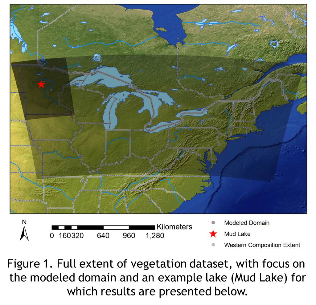
Using North American Regional Reanalysis (NARR) wind data, a vegetation dataset of tree composition pre-Euro-American settlement , fossil pollen records from the Neotoma Paleoecology Database, and taxon-specific measurements of settling velocities for pollen grains, we are producing improved estimates of pollen loading (in grains per square meter) for lakes across the Prairie-Forest ecotone in the upper Midwest.  This work recently won an Outstanding Student Paper Award from the 2014 Fall Meeting of the American Geophysical Union.

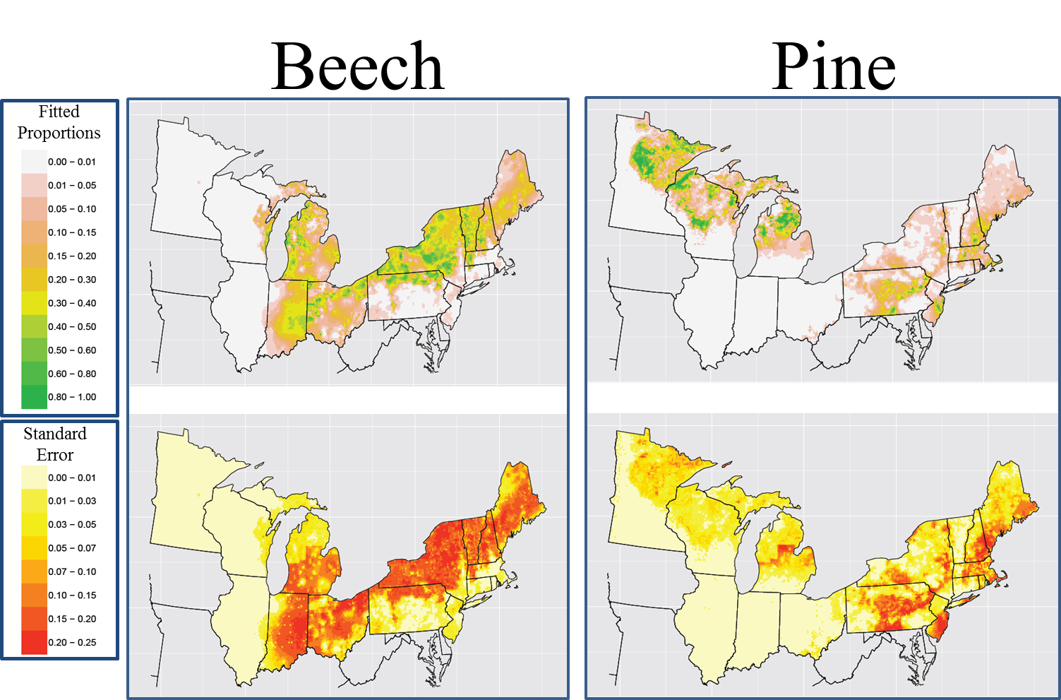
While the source area is largely governed by presence/absence of taxa in the vegetation dataset, things become much more interesting when looking at the ratio of relative proportion of pollen loading to relative proportion of trees per grid cell. We see that some taxa are much better represented in the pollen records given the number of trees on the landscape.

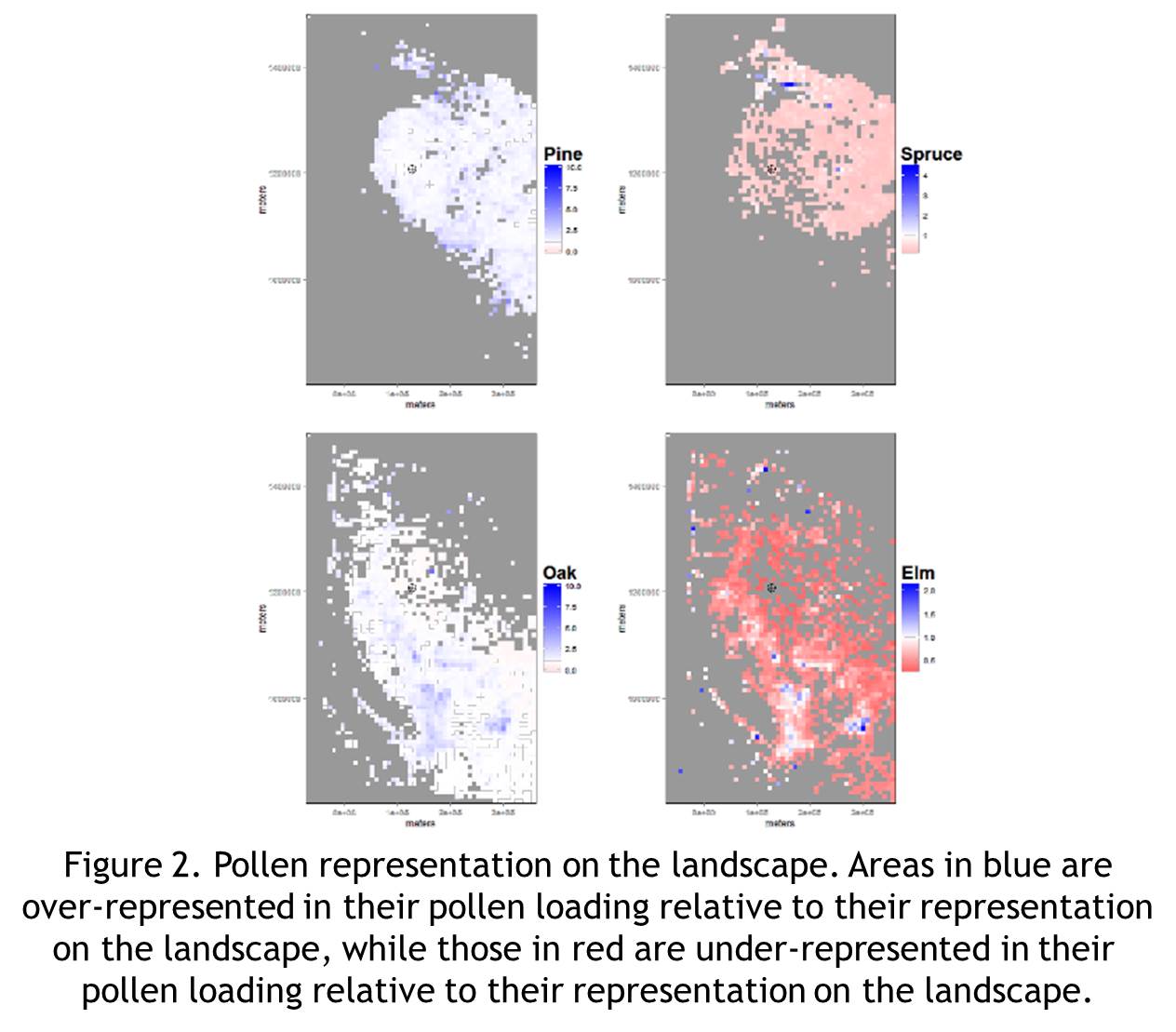
We can also see that whether a given taxon is over- or underrepresented varies spatially, based on distance to lake and the other taxa present in a given grid cell.  These results shed light on the potential magnitude of a regional pollen source area, and help elucidate the relationship between pollen in a sediment core and trees on the landscape.  Ultimately, this kind of work can be used to build more accurate reconstructions of past vegetation from fossil pollen records.  From there, these paleovegetation reconstructions can be used to better constrain and improve terrestrial ecosystem models – a central goal of the PalEON project.

To see more results, including preliminary comparisons to pollen counts from sediment cores, you can check out our American Geophysical Union poster here.

References:

1. Fries, M. Review of Palaeobotany and Palynology, 1967.
2. Marquer et al. Quaternary Science Reviews, 2014.
3. Prentice, C. Quaternary Research, 1985.
4. Sugita, S. Quaternary Research, 1993.

Post by Andria Dawson, Post-Doc at University of California-Berkeley

Pollen and seed dispersal are important reproductive processes in plants, and in part determines the abundance and extent of a species. With a recent push to understand how species will respond to global climate change, dispersal ecology has gained increasing interest. We really want to know if there is a dispersal limitation, or if species can migrate quickly enough to maintain survival in a changing environment. Addressing this question presents challenges, many of which arise from trying to understand and quantify dispersal in ecosystems that are changing in both space and time (Robledo-Arnuncio 2014).

In PalEON, one of our efforts involves estimating the past relative abundance of vegetation from fossil pollen records. To do this, we need to quantify the pollen-vegetation relationship, which includes modelling pollen dispersal processes.

For many trees, including those we study in the PalEON domain, pollination is exclusively (or at least predominantly) anemophilous (carried out by wind). In angiosperms, wind pollination is thought to have evolved as an alternative means of reproduction for use when animal pollinators are scarce (Cox 1991). It was previously understood that wind pollination was less efficient than insect pollination (Ackerman 2000), but Friedman and Barrett (2009) show that may not be the case. To estimate the efficiency of wind pollination, they compared pollen captured by stigmas to pollen produced, and found that the mean pollen capture was about 0.32%, which is similar to estimates of animal pollination efficiency. Although both dispersal vectors are comparable with respect to efficiency, these quantities indicate that both are still pretty inefficient – this is great news for paleoecologists! Some of the pollen that is not captured ends up in the sediment.

Now we know that we expect to find pollen in the sediment, but how do we begin to quantify how much pollen of any type we expect to find at a given location? The route a pollen grain takes to arrive at its final location is governed by atmopsheric flow dynamics (among other things). These dynamics are complicated by landscape heterogeneity and climate, and differ among and within individuals because not all pollen grains are created equal. However, we usually aren’t as interested in the route as we are in the final location – in particular, we want to know the dispersal location relative to the source location. The distributions of dispersal locations from a source defines a dispersal kernel which can be empirically estimated with dispersal location data. Often these kernels are modelled using parametric distributions, usually isotropic, and often stationary with respect both space and time. Are these approximations adequate? If so, at what scale? These are some of the questions we hope to address by using Bayesian hierarchical modelling to quantify the pollen vegetation relationship in the Upper Midwest.

References
1. Robledo-Arnuncio, JJ, et al. Movement Ecology, 2014.
2. Cox, PA. Philosophical Transactions of the Royal Society B: Biological Sciences, 1991.
3. Friedman, J, Barrett SCH. Annals of Botany, 2009.
4. Ackerman, JD. Plant Systematics and Evolution, 2000.

Posted by Jody Peters

The crew at Notre Dame is in the process of entering PLS data for Indiana. Recently we focused on the area around Notre Dame and South Bend. Here is the area as depicted in the 1829 PLS survey, 13 years before Notre Dame’s founding.
It has been interesting to learn about the changes that have taken place around campus. While the major roads around Notre Dame (Angela, Douglas and Juniper) were originally based off the PLS survey, all three roads have had sections of them moved.

In the 1829 survey, the two lakes on campus were drawn as one. We aren’t sure if this is because the surveyor was in a hurry and didn’t take time to explore the lakes further or if he was surveying in the winter when the lakes were ice covered. But from historical documents at Notre Dame there are a number of references to two lakes, although the lakes water levels have been known to fluctuate and at some points were quite high making the area between the lakes quite swampy.
At the time of the PLS survey the Notre Dame area was dominated by oaks. But another tree found in the area that was of interest to the lab was the pepperage tree. The pepperage tree, or more commonly spelled, pepperidge is also known as sour gum, black gum or black tupelo. As a side note, the pepperidge tree is where Pepperidge Farms get their name (got to love those goldfish crackers)! To learn more about pepperidge trees, check out this great site. Keep up to date with ND’s data entry progress by clicking on Indiana map at our Settlement Vegetation Site.

References

[1] Updated citation as of 4-17-14:Lutz, David A., Howarth, Richard B., “Valuing albedo as an ecosystem service: implications for forest management. Climatic Change (2014): doi:10.1007/s10584-014-1109-0
Original citation: Dartmouth College. “Can cutting trees help fight global warming? More logging, deforestation may better serve climate in some areas, study finds.” ScienceDaily. ScienceDaily, 5 December 2013.
[2] Keenan, Trevor F., et al. “Increase in forest water-use efficiency as atmospheric carbon dioxide concentrations rise.” Nature 499.7458 (2013): 324-327.
[3] Spracklen, Dominick V., Boris Bonn, and Kenneth S. Carslaw. “Boreal forests, aerosols and the impacts on clouds and climate.” Philosophical Transactions of the Royal Society A: Mathematical, Physical and Engineering Sciences 366.1885 (2008): 4613-4626.
[4] Dale, Virginia H., et al. “Climate Change and Forest Disturbances Climate change can affect forests by altering the frequency, intensity, duration, and timing of fire, drought, introduced species, insect and pathogen outbreaks, hurricanes, windstorms, ice storms, or landslides.” BioScience 51.9 (2001): 723-734.
The Invasion of the Zombie Maples
Post by Ana Camila Gonzalez, Undergraduate Researcher with Neil Pederson and the Tree Ring Laboratory at Columbia’s Lamont-Doherty Earth Observatory
As an undergraduate student interning at the Tree Ring Lab at Lamont-Doherty Earth Observatory, my involvement with PalEON has been rather localized to the data production side of things. My knowledge on the dynamics of climate and the models involved in forecasting future climate change is obviously limited as a second-year student. My knowledge on how frustrating it can be to cross-date the rings in Maple trees, however, is more extensive.
This past summer I was able to join the Tree Ring Lab on a fieldwork trip to Harvard Forest in Petersham, MA. My main task was to map each plot where we cored, recording the species of each tree cored, its distance to the plot center, its DBH, its canopy position, its compass orientation, and any defining characteristics (the tree was rotten, hollow, had two stems, etc.). The forest was beautiful, but it became more beautiful every time I wrote down the letters QURU (Quercus rubra)I had plenty of experience with oaks, and knew that they did not often create false or missing rings and are thus a fairly easy species to cross-date. I shuddered a little every time I had to write down BEAL (Betula alleghaniensis), however, since I had looked at a few yellow birches before and knew the rings were sometimes impossible to see let alone cross-date. I had no reaction to the letters ACRU (Acer rubrum), however, since I had never looked at a red maple core before. I was happy that it was a tree I could easily identify, and so I didn’t mind that the letters kept coming up. Had I known what was to come, I would’ve found a way to prevent anyone from putting a borer to a red maple.
At first, the maples seemed to be my friends. The rings were sensitive enough that multiple marker years helped me figure out where the missing rings where, what was false and what was real. I morbidly became a fan of the gypsy moth outbreak of 1981, because in many cases (but not all) it produced a distinct white ring that marked that year very clearly. This was definitely challenging, as the trees also seemed to be locally sensitive (a narrow ring in one tree might not at all be present in another) but all in all it seemed to be going well.
And then came the Zombie Maples.
Fig (a) Anatomy of a White Ring: Above is a core collected in 2003. It was alive. The white ring in the center of the image is 1981, the year of the regional gypsy moth outbreak in New York and New England.
That white ring you’re seeing above is the characteristic 1981 ring from a Zombie Maple cored in 2003. After that ring we can only see four rings – but this tree is alive, which means that there should be 13 rings after 1990 (Fig b). This means approximately 10 are missing.
Fig (b) Anatomy of a Zombie Maple: Above is a core collected in 2003. It was alive. The 1990 ring is marked in the image just right of center. There should be 13 rings between 1990 and the bark. You can only see four. Is it Alive? Is it Dead? Eek! It is a Zombie!!
This kind of suppression in the last two decades was present in multiple cores, and it made many perfectly alive trees seem like they should have been dead. Nine rings missing in a little over one millimeter. We see even more severe cases in our new collection: 15 rings where there should be 30 rings in about 2 millimeters – how is this tree supporting itself?
Cross-dating these cores took a lot longer than planned, and at times I was tempted to pretend my box of maples went missing, but afterwards I felt I was a much stronger cross-dater, and I’m realizing more and more that this really matters. If you’re going to base a model off of data that involves ring-width measurements from particular years, you better make sure you have the right years. What if we didn’t know the gypsy moth outbreak occurred in 1981, and somebody counting the rings back on the Zombie maple core above was led to believe it occurred in 1996? Our understanding of the trigger for this event would be incorrect because we would be looking for evidence from the wrong decade.
In a way, the Maples are still my friends. They were almost like the English teacher in high school who graded harshly who you didn’t appreciate until you realized how much better your writing had become.
PLS around Notre Dame