Post by Kelly Heilman, a graduate student with Jason McLachlan at the University of Notre Dame

If trees could talk…

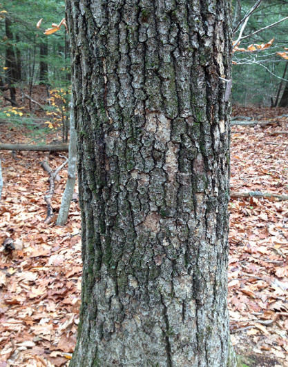
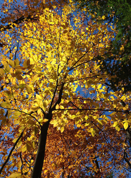
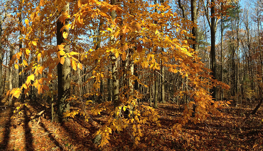
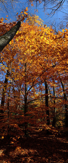
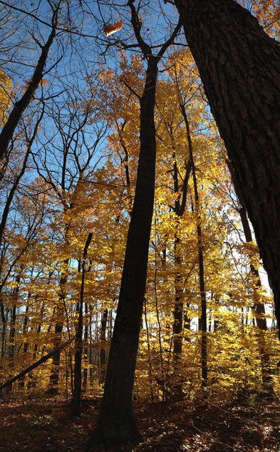
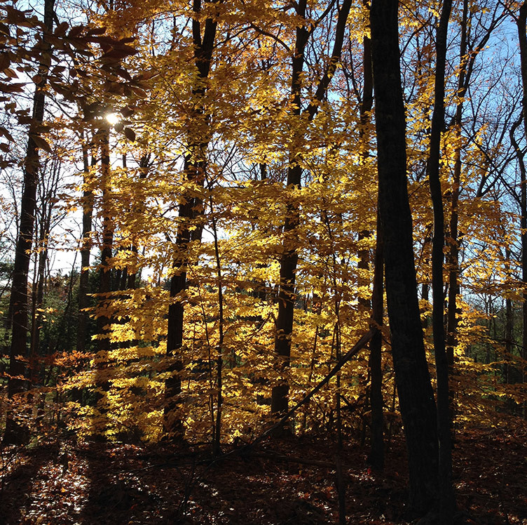
Every year, oak trees in the Midwest awaken in spring, to spread their leaves to grow through the summer, and settle down for a long winter’s rest in the fall. As we watch this seasonal cycle, trees warn us of the coming of winter as they shed their leaves, putting on a glorious show of red, gold and orange. At times, trees tell us to slow down by inviting us into their expansive shade to rest, read a book, and listen the birds sing in the distance. However, to many dendrochronologists, trees talk about something else–their records of the past. The patterns of each season’s tree growth are recorded in the annual rings of trees, and are protected like a memory beneath the tree’s bark. These annual variations in tree rings provide researchers with information on the responses of trees to climate variations, as well as to other stresses that trees face, such as competition with their neighbors for light, and fire disturbances. All this makes tree ring records particularly useful tools for looking into the past. So, in a way trees can talk . . . but it takes some effort for us to listen to them.

Trees in the temperate zone, such as this Bur Oak, record annual rings of growth, allowing us to count their rings to get tree age, and correlate growth with climate records. Pictured above is a 5-mm wide core sample from a tree at Bonanza prairie SNA (Scientific and Natural Area) in Minnesota, with the bark pictured on the left and the center of the tree on the right. (Click on image for a larger view.)

Looking at the past responses of ecosystems to climate variations through the lens of tree rings can provide a better understanding of how these ecosystems might respond to future changes. My research focuses broadly on the savanna-forest boundary in the Midwest, both on the environmental conditions that form this boundary and how environmental changes impact these savannas and forests. Over the last century, humans have altered the landscape in the Midwest, through large scale agriculture, land-use change, fire suppression, changes in CO₂ and climate shifts (Goring et al. 2016, Rhemtulla et al. 2007). Many of these changes have likely affected the growth, survival, and climate sensitivity of trees, which could impact the trajectory of forests in the future. Therefore, I set out to quantify how savanna and forest trees functioned both in the past, and on the modern landscape. Using annual growth increments recorded in tree rings, my objective was to quantify how both modern and past ecosystems functioned (in terms of how much carbon they uptake and store in their annual growth rings), and to determine if and how tree growth patterns vary across temperature, precipitation, and soil gradients.

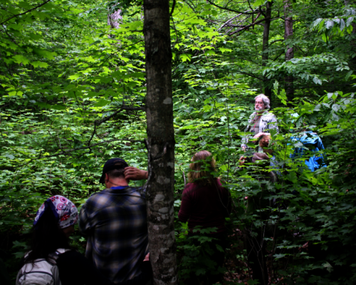
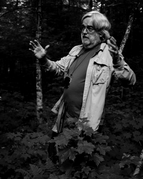
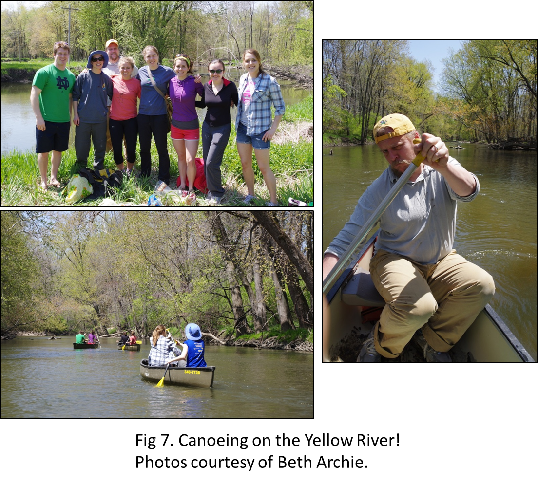
Thoughts from the field (don’t forget your bug spray and sunscreen):

To view the annual rings of tree growth, we collected tree core samples from sites across the historic savanna-forest boundary in the Midwest from several Minnesota Scientific and Natural Areas (SNAs), Minnesota State Parks, State Parks in Iowa and Missouri, as well as several sites within McHenry County Conservation District in Illinois (see map). In my sampling design, I aimed to capture the growth responses of young and old trees in both savannas and forests, across the wet-to-dry climate gradient in the Midwest. We targeted several Oak species, including Bur Oak (Quercus macrocarpa), White Oak (Quercus alba), Red Oak (Quercus rubra), and Chinkapin Oak (Quercus muehlenbergii), but also sampled several eastern forest species as well. With the help of fellow Paleonistas (Ann Raiho, Monika Shea) and field technicians Evan Welsh and Santi Thompson, we sampled tree cores at 23 different sites during the summers of 2015 and 2016. Coring trees can be monotonous, physically difficult, and relaxing all at the same time. Lucky for us, we got to go to some beautiful places across the Midwest.

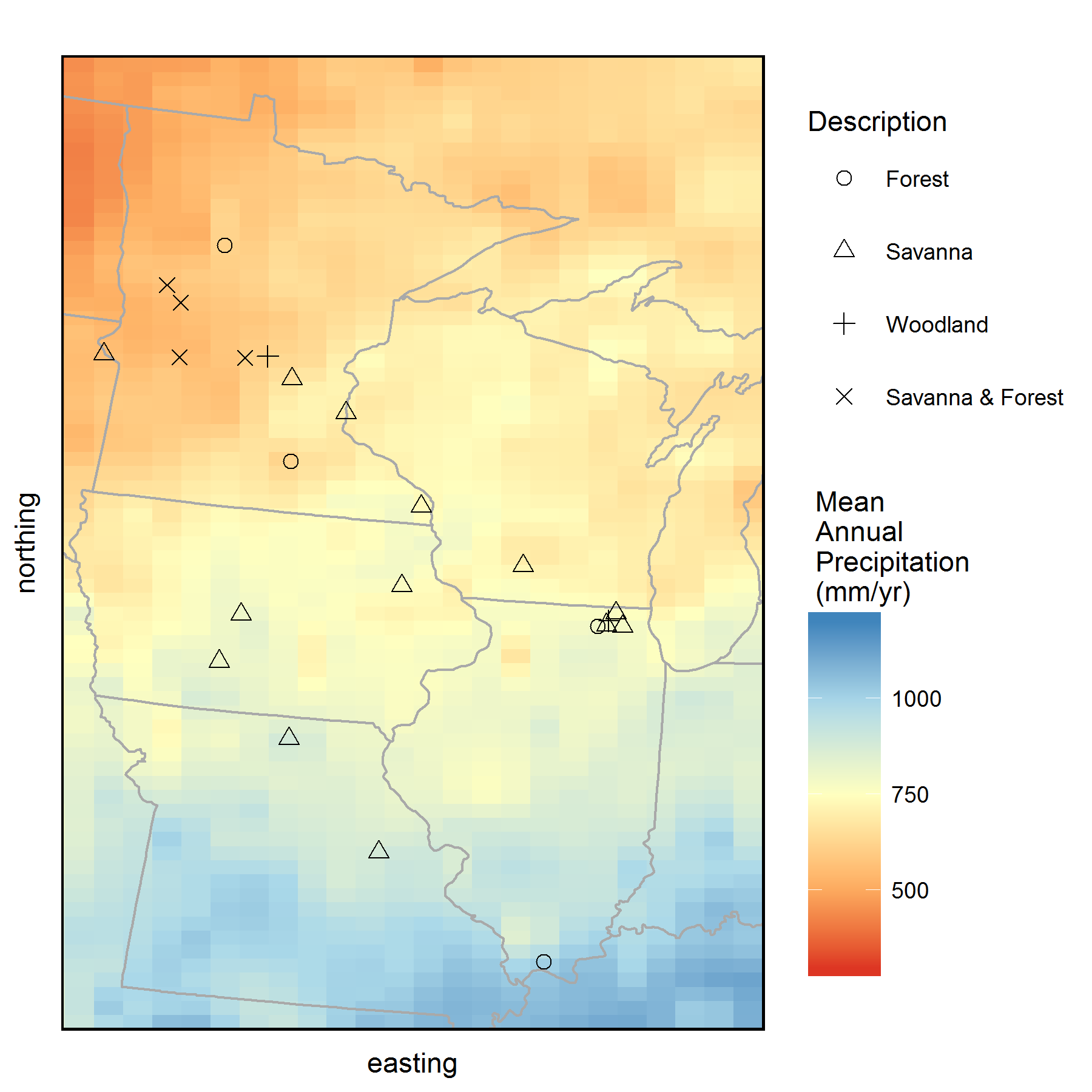
Map of all the sites where we collected tree core samples from during 2015 and 2016. Background color represents mean annual precipitation (MAP) of the region obtained from PRISM climate data. Tree cores were collected from savannas and forests that occur along the historic prairie-forest boundary in the Midwest. (Click on image for a larger view.)

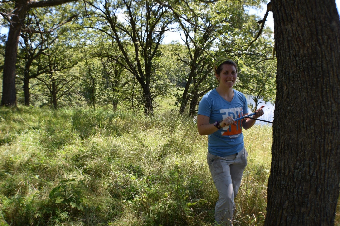
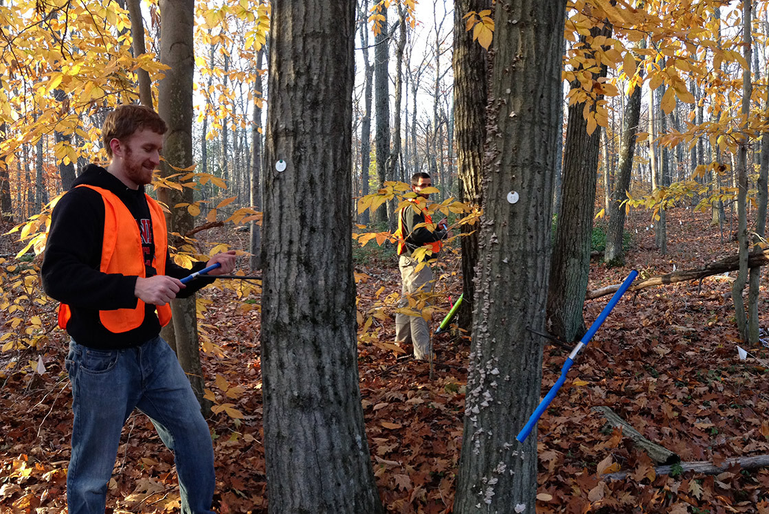
Coring a large Bur Oak tree in a savanna at Maplewood State Park, Minnesota.

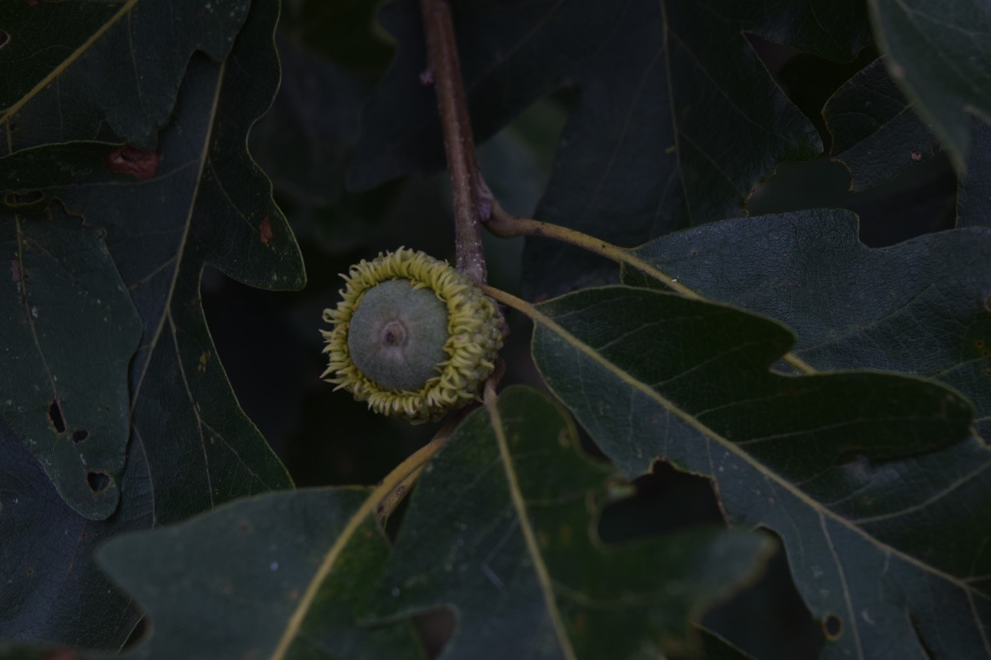
Bur Oak acorn from a young tree located in St. Croix savanna SNA in Minnesota

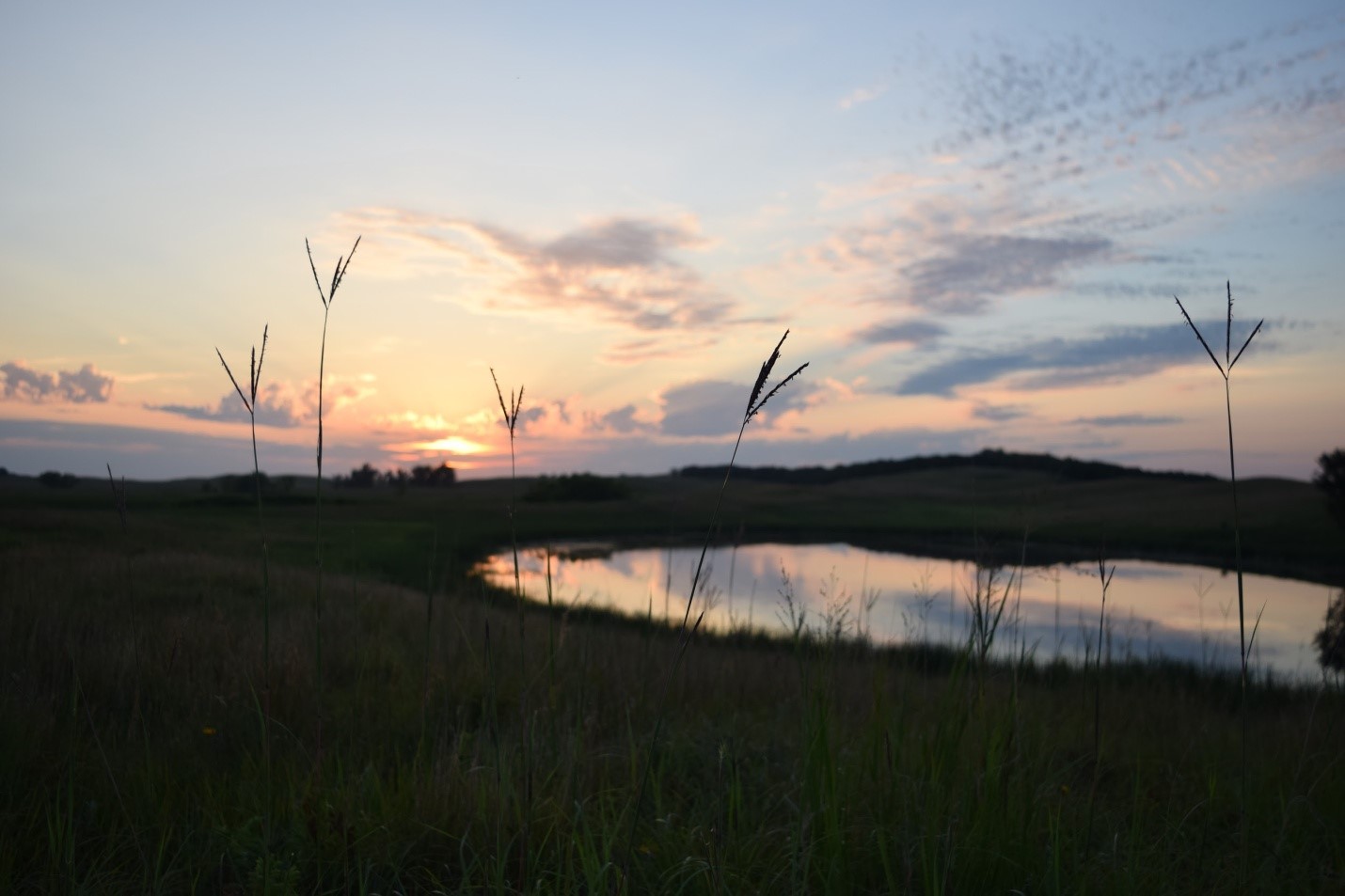
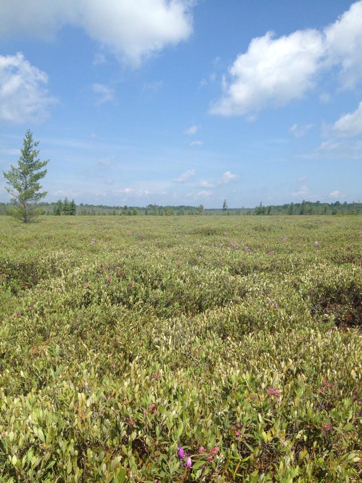
Working out in the field gave us opportunities to see some awesome ecosystems and sunsets. Looking out onto to prairie from a savanna at Glacial Lakes State Park, MN, the tallest plants were not trees, but tallgrass prairie plants, such as the Big Bluestem, or “turkey foot” (Andropodon gerardii) pictured here.

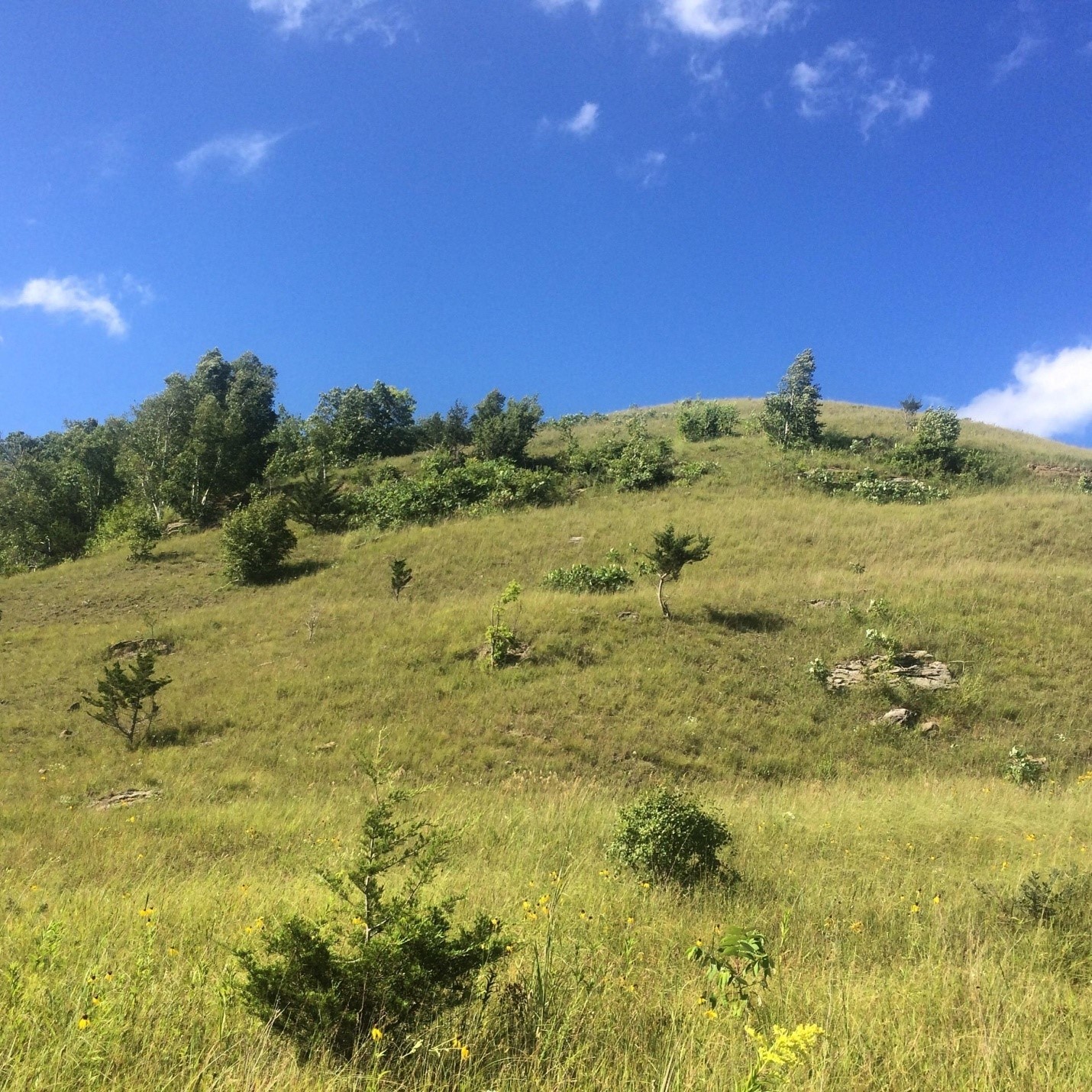
An open savanna and prairie complex at Mound Prairie SNA, in Minnesota.

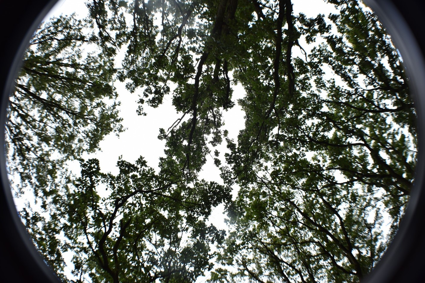
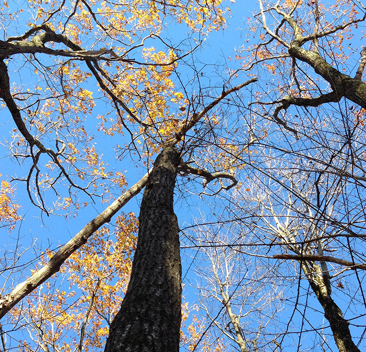
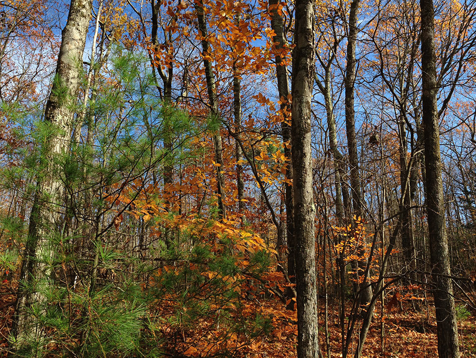
The Oak savanna canopy is sparse compared to a closed forest, letting in plenty of light for understory grasses and forbs to grow.

After driving a couple thousand miles total, spending over 30 nights in a tent in 2015 and 2016, and battling what seemed like an infinite amount of mosquitoes and ticks, we headed back to the lab to measure the width of each annual tree ring, and determine how climate affects Midwestern oak tree growth.

Back at the Lab:

Once we returned from the field, the cores were glued to wooden mounts, sanded, counted and measured. This work was done with the help of several awesome undergraduate students over the last two years, including: Jacklyn Cooney, Clare Buntrock, Santi Thompson, and Da Som Kim. Once the cores were measured and cross-dated with each other (using common “marker” years of extremely low growth, such as the 1934 Dust bowl drought, to double check our measurements), we have a temporal record of growth fluctuations for each site.

What climate factor affects oak tree growth in savannas and forests?

Tree growth responds strongly to the most limiting factor to their growth.

http://www.newyorker.com/cartoon/a19671

For example, in water limited regions of Southwestern North America, tree growth is highly correlated with interannual precipitation and drought, often making tree ring records from these regions good candidates for precipitation reconstructions (Charney et al. 2016, Peterson 2014). However, in many Eastern North American forests, water availability for growth is not a huge limiting factor, and tree growth is more sensitive to summer temperatures, drought, and light availability (Peterson 2014, Charney et al. 2016).  The savanna-forest boundary in the Midwest is located between these Eastern closed forests and the more water limited prairies to the West. Therefore, tree species that occur along this boundary are often thought to exist at the edge of their theoretical and climatic range boundaries, and theoretically could respond strongly to moisture stress or temperature stress. The historic transition from open prairie to savanna to forests occurred at a range of precipitation and temperature climatic envelopes; this transition zone in Minnesota had low mean annual precipitation (300-600 mm/year), and much higher mean annual precipitation in Indiana & Illinois (700-1200). Therefore, I originally hypothesized that these western savannas and forests may respond more strongly to low precipitation and drought than Eastern savannas and forests.

Contrary to my original hypotheses, oak tree ring growth is not primarily controlled by precipitation in oak trees near the savanna-forest boundary. Rather, tree growth at most sites is strongly linked to summer drought severity and summer temperatures. The negative impacts of drought on tree ring growth are likely mediated by temperature-induced drought stress, as suggested by the strong negative correlations with minimum and maximum June and July temperatures at almost all sites. While growth at some sites is mildly correlated to late summer precipitation, these places tend to have sandy soils, suggesting that future decreases in precipitation could have larger negative consequences for tree growth on sites with sandy soils. Interestingly, despite low moisture availability, sites with the lowest mean annual rainfall were only weakly correlated with monthly precipitation, suggesting that perhaps these systems are relying heavily on deeper groundwater sources for water. However, sites with low rainfall, such as Bonanza Prairie SNA in Minnesota, do have strong sensitivity to drought indices (Palmer Drought Severity Index, PDSI) and temperature indicating that high temperature drought stress, rather than water stress due to low precipitation is more important in this ecosystem.

Correlations with monthly climate indicate that Oak trees at most sites are most sensitive to summer drought index and summer temperatures, but few are strongly sensitive to monthly precipitation. Red colored sites have lower mean annual precipitation, and blue sites have higher mean annual precipitation. A). Tree growth at all sites is most strongly correlated to summer drought (Palmer Drought Severity Index is positive in non-drought periods and negative in drought periods). B). July precipitation is only weakly correlated with growth at some sites. C). Tree growth is somewhat negatively correlated with summer maximum temperatures. (Click on image for a larger view.)

Have growth sensitivities changed over time?

The climate-growth relationship is often assumed to be constant for the purposes of climate reconstructions. However, recent dendroecological studies recognize that growth-climate relationships may change due to shifts in climate seasonality, changes in tree size class, tree competition, and possibly due to increases in atmospheric CO₂ (Voelker et al. 2006). In theory, higher levels of CO₂ in the atmosphere can enhance tree growth by increasing CO₂ available for photosynthesis in the leaf, without changing stomatal conductance (g_s, the amount of water that moves through the stomata). This results in an increase in plant Water Use Efficiency (WUE), or the amount of carbon taken up per unit of water used, which could help reduce the impacts of drought on trees (McCarroll and Loader 2004). While the effect of atmospheric CO₂ on tree growth is still largely debated, past researchers found that Bur Oak (Quercus macrocarpa) trees in Western Minnesota have become less sensitive to drought since the beginning of the 20th century, and mortality due to drought has decreased  as well (Wyckoff and Bowers 2009). Additionally, Voelker et al. (2006) found that the positive effects on growth that may result from increased atmospheric CO₂ likely decline with tree age. My sampling effort has extended the spatial range of oak sampling in the Midwest, allowing us to test whether a change in the growth–drought relationship over the 20^th century is regional and if it has occurred in different oak species and site conditions.

With our data across the Midwest, we find preliminary evidence supporting a change in growth sensitivity to climate. Trees across the Midwest were less sensitive to drought after 1950, and younger trees established under high CO₂ were also less sensitive to drought than older trees.

These results are consistent with the previous work in Minnesota (Wyckoff and Bowers 2009), and with a positive enhancement of CO₂. In two of the three closed forest sites sampled, we find no difference in the growth-drought sensitivity over time, suggesting that savanna trees, but not forest trees have become less susceptible to drought in the region. While the stand structure (open savanna or closed forest) may help explain where we see shifts in growth-climate sensitivity, species sampled may also play a role, as well as the mean annual precipitation and temperature. To specifically test whether CO₂ enhancement is driving the decreased drought sensitivity, I am currently working on a project that tests to see if the composition of carbon isotopes recorded within annual tree rings have changed. The ratio of heavy to light carbon isotopes can be used to quantify plant Water Use Efficiency, which will increase over time if CO₂ has a net positive effect on tree growth.

Up Next…

This project is still ongoing and there are several questions that I am still exploring. I am continuing to work on a formal analysis of the tree ring growth data, and look more at species-specific sensitivities to climate, since the preliminary analyses focus on site specific responses.

If growth and sensitivity of growth to climate changes over time, I want to know if it is due to the effects of CO₂, or some other factor affecting forest growth. This next year, I will be spending a lot of time in the lab quantifying stable carbon isotopes, to determine if plant WUE increases result in the decrease in drought sensitivity over time.

References:
Charney, N. D., et al. (2016). Observed forest sensitivity to climate implies large changes in 21st century North American forest growth. Ecology Letters, 19(9), 1119–1128. https://doi.org/10.1111/ele.12650

Goring, S. J., et al. (2016). Novel and Lost Forests in the Upper Midwestern United States, from New Estimates of Settlement-Era Composition, Stem Density, and Biomass. PLOS ONE, 11(12), e0151935. https://doi.org/10.1371/journal.pone.0151935

McCarroll, D., & Loader, N. J. (2004). Stable isotopes in tree rings. Quaternary Science Reviews, 23(7–8), 771–801. https://doi.org/10.1016/j.quascirev.2003.06.017

Peterson, D. L. (2014). Climate Change and United Steates Forests. In Climate Change and United States Forests. Springer. Retrieved from http://www.springer.com/us/book/9789400775145

Rhemtulla, J. M., et al. (2007). Regional land-cover conversion in the U.S. upper Midwest: magnitude of change and limited recovery (1850–1935–1993). Landscape Ecology, 22(1), 57–75. https://doi.org/10.1007/s10980-007-9117-3

Voelker, S. L., et al. (2006). Historical CO2 Growth Enhancement Declines with Age in Quercus and Pinus. Ecological Monographs, 76(4), 549–564.

Wyckoff, P. H., & Bowers, R. (2010). Response of the prairie–forest border to climate change: impacts of increasing drought may be mitigated by increasing CO2. Journal of Ecology, 98(1), 197–208. https://doi.org/10.1111/j.1365-2745.2009.01602.x

Posted by Jody Peters, PalEON Program Manager

Prior to major land use changes, the tall grass prairie was a widespread ecotone in North America extending east into Minnesota, Illinois and Indiana.  Caitlin Broderick, a

Figure 1. Study area. Townships within the Yellow River watershed.

University of Notre Dame undergraduate working in the McLachlan lab, wanted to learn more about the edge of the prairie this spring semester.  She could have listened to NPR’s Garrison Keillor describe life in Lake Wobegone on the edge of the prairie in Minnesota.  But given that Notre Dame has been compiling historical records of trees from Indiana and Illinois, she decided to look at bit closer to home and focused on townships that are within the Yellow River watershed.  Coincidentally, this watershed is split almost in two by what is currently US 31 and what was historically known in the Public Land Survey (PLS) notes as the Michigan Road Lands. (Fig 1).

The following are some of the results Caitlin presented at the University of Notre Dame College of Science Joint Annual Spring Meeting.

Currently, the Yellow River region is dominated by agriculture and deciduous forests (Fig 2).  However, from a 1935 depiction of the extent of the prairie prior to Euro-American settlement, prairie ecosystems extended into northwest Indiana including into the Yellow River region (Fig 3; Transeau 1935).  Caitlin explored what the edge of the prairie in the Yellow River region looked like during 1829-1837 using historical forest data obtained from PLS.The survey notes provide identification of 1-2 trees, their diameters and distances from corner posts set every mile in each township (n=30 townships; 1055 corners). For this study, trees at each corner were categorized as “Oak” (only oaks were present), “Other” (22 non-oak tree taxa which were dominated by beech, ash, maple and elms), or “Oak + Other” (a combination of oak and non-oak trees).  There were also corners that were categorized as “Water” (in lakes, rivers, creeks, etc.), “No Tree” (had a post set in a mound but with no trees nearby), or “No Data” (corners with no information provided in the notes).

Caitlin used Arc GIS to map the tree composition at each corner (Fig 4).  Much to our surprise, she did not see many corners with no trees in the areas of Transeau’s prairie in the Yellow River region.  However, there was a striking pattern in the distribution of the trees, with the majority of the trees to the west of the Michigan Road Lands being oaks and those to the east being other hardwoods.

In addition to examining tree composition, Caitlin wanted to look at the structure of the trees and the physical environment across the region. To better define the two groups of trees (Oaks to the west and Other hardwoods to the east), Caitlin created buffers around individual corners and dissolved the buffers with matching tree classifications to create two groups of trees (Fig 5A). Comparing the trees in the two groups, Caitlin found that there was no difference in tree diameter (mean (cm)± se; Oak: 40.9± 0.5; Other: 40.2± 0.6). However, the trees in the Oak group were significantly further from the corner posts compared to the Other group (mean (m)± se; Oak: 36.2± 4.3; Other: 13.6± 2.4; p<0.001).  Given that there was a difference in the tree composition and distance from the corners, Caitlin looked at climatic and physical features that could help explain this difference between the oaks of the west and the other hardwoods in the east.  There was no ecological difference in either temperature or precipitation (mean± se; Temperature (ºC): Oak: 9.88± 0.003; Other: 9.89± 0.003; Precipitation (mm): Oak: 1010± 0.59; Other: 1007± 0.74).  However, although northern Indiana is quite flat, as with the tree composition, there was a striking difference in the pattern of elevation change across the Yellow River region that mirrored the change in the tree distribution. Trees in the Oak group were at significantly lower elevation compared to trees in the Other group (mean (m)± se; Oak: 225.5± 0.7, Other: 251.0± 0.6; p<0.01; Fig 5B).

In addition to exploring what the historical prairie-forest boundary looked like, Caitlin compared the National Commodity Crop Productivity Index (NCCPI) to see if there is a lasting impact on the current crop production by the physical factors that contributed to the differences in historical tree composition and structure.  The NCCPI models the ability of soils, landscapes, and climates to foster non-irrigated commodity crop productivity (Dobos et al. 2012). Caitlin found there was in fact, a difference between NCCPI of the two groups with crop productivity being significantly lower in the western area historically dominated by low density Oak tree communities (Fig 6).

Typically when people think of prairies, they think of open expanses of grass.  However, over the spring semester Caitlin found that in the Yellow River region of northern Indiana, the prairie described by Transeau actually looked more like a low density oak community compared to the closed forests further east.  While at first glance we can no longer see the prairie’s edge in the current vegetation of northern Indiana (Fig 2), when Caitlin looked closer, the factors that once controlled the boundary between the closed forests of the east and the open savannas moving west may still be at work limiting crop production in what was once savanna compared to production in the historically wooded uplands (although what these factors specifically are is still an open question).

As a fun follow-up to Caitlin’s research, nine of us took a lab canoe trip down the Yellow River. Although we didn’t see the same striking pattern of oaks to the west and other hardwoods to the east, as we drove the 50 minutes south on US 31 to get to the River, we did see small stands of hardwoods intermingled with a number of lone oaks standing in the middle of corn and soybean fields.  On our way to the ice cream store after our canoe trip, we also saw some of the lasting impacts of the oak savannas as we drove through Burr Oak, Indiana.  According to McDonald (1908), the village plat was filed in 1882 and was “nearly in the center of what is known as the “Burr Oak Flats”, which is as beautiful and productive a region as can be found anywhere.”

The trip down the Yellow River was a wonderful way to get outside on a beautiful spring day and experience firsthand the watershed/ecosystem that Caitlin has spent this spring studying in the lab.  The river was an easy enough paddle that novice canoers would be comfortable, but had enough downed trees to provide excitement for the more experienced canoer.  If you are ever in the area, connect with the Little Bit Canoe Rental. They do a wonderful job providing canoes and transport. Here are a couple of pictures of the fun!

References

Dobos, R.R., H.R. Sinclair, Jr., M.P. Robotham. 2012. User Guide for the National Commodity Crop Productivity Index (NCCPI), Version 2.0. Access pdf at the bottom of the page here.

McDonald, D. 1908. A Twentieth Century History of Marshall County, Indiana, Volume 1. Lewis Publishing Company, pg 134. Online access here.

Transeau, E. N. 1935. The Prairie Peninsula. Ecology 16(3): 423-437.

Post by Ana Camila Gonzalez, Undergraduate Researcher with Neil Pederson and the Tree Ring Laboratory at Columbia’s Lamont-Doherty Earth Observatory

As an undergraduate student interning at the Tree Ring Lab at Lamont-Doherty Earth Observatory, my involvement with PalEON has been rather localized to the data production side of things. My knowledge on the dynamics of climate and the models involved in forecasting future climate change is obviously limited as a second-year student. My knowledge on how frustrating it can be to cross-date the rings in Maple trees, however, is more extensive.

This past summer I was able to join the Tree Ring Lab on a fieldwork trip to Harvard Forest in Petersham, MA. My main task was to map each plot where we cored, recording the species of each tree cored, its distance to the plot center, its DBH, its canopy position, its compass orientation, and any defining characteristics (the tree was rotten, hollow, had two stems, etc.). The forest was beautiful, but it became more beautiful every time I wrote down the letters QURU (Quercus rubra)– I had plenty of experience with oaks, and knew that they did not often create false or missing rings and are thus a fairly easy species to cross-date. I shuddered a little every time I had to write down BEAL (Betula alleghaniensis), however, since I had looked at a few yellow birches before and knew the rings were sometimes impossible to see let alone cross-date. I had no reaction to the letters ACRU (Acer rubrum), however, since I had never looked at a red maple core before. I was happy that it was a tree I could easily identify, and so I didn’t mind that the letters kept coming up. Had I known what was to come, I would’ve found a way to prevent anyone from putting a borer to a red maple.

At first, the maples seemed to be my friends. The rings were sensitive enough that multiple marker years helped me figure out where the missing rings where, what was false and what was real. I morbidly became a fan of the gypsy moth outbreak of 1981, because in many cases (but not all) it produced a distinct white ring that marked that year very clearly. This was definitely challenging, as the trees also seemed to be locally sensitive (a narrow ring in one tree might not at all be present in another) but all in all it seemed to be going well.

And then came the Zombie Maples.

Fig (a) Anatomy of a White Ring: Above is a core collected in 2003. It was alive. The white ring in the center of the image is 1981, the year of the regional gypsy moth outbreak in New York and New England.

That white ring you’re seeing above is the characteristic 1981 ring from a Zombie Maple cored in 2003. After that ring we can only see four rings – but this tree is alive, which means that there should be 13 rings after 1990 (Fig b). This means approximately 10 are missing.

Fig (b) Anatomy of a Zombie Maple: Above is a core collected in 2003. It was alive. The 1990 ring is marked in the image just right of center. There should be 13 rings between 1990 and the bark. You can only see four. Is it Alive? Is it Dead? Eek! It is a Zombie!!

This kind of suppression in the last two decades was present in multiple cores, and it made many perfectly alive trees seem like they should have been dead. Nine rings missing in a little over one millimeter. We see even more severe cases in our new collection: 15 rings where there should be 30 rings in about 2 millimeters – how is this tree supporting itself?

Cross-dating these cores took a lot longer than planned, and at times I was tempted to pretend my box of maples went missing, but afterwards I felt I was a much stronger cross-dater, and I’m realizing more and more that this really matters. If you’re going to base a model off of data that involves ring-width measurements from particular years, you better make sure you have the right years. What if we didn’t know the gypsy moth outbreak occurred in 1981, and somebody counting the rings back on the Zombie maple core above was led to believe it occurred in 1996? Our understanding of the trigger for this event would be incorrect because we would be looking for evidence from the wrong decade.

In a way, the Maples are still my friends. They were almost like the English teacher in high school who graded harshly who you didn’t appreciate until you realized how much better your writing had become.