Identifying Local Fire Events From Sediment Charcoal Records Via Regularization

Post by Malcolm Itter, a graduate student with Andrew Finley at Michigan State University. Malcolm received an Outstanding Student Paper Award for this work at AGU 2016!

Charcoal particles deposited in lake sediments during and following wildland fires serve as records of local to regional fire history. As paleoecologists, we would like to apply these records to understand how fire regimes, including fire frequency, size, and severity, vary with climate and regional vegetation on a centennial to millennial scale. Sediment charcoal deposits arise from several sources including: 1) direct transport during local fires; 2) surface transport via wind and water of charcoal deposited within a lake catchment following regional fires; 3) sediment mixing within the sample lake concentrating charcoal in the lake center. A common challenge when using sediment charcoal records is the need to separate charcoal generated during local fire events from charcoal generated from regional and secondary sources. Recent work by PalEON collaborators including myself, Andrew Finley, Mevin Hooten, Phil Higuera, Jenn Marlon, Ryan Kelly, and Jason McLachlan applies statistical regularization to separate local and regional charcoal deposition allowing for inference regarding local fire frequency and regional fire dynamics. Here we describe the general concept of regularization as it relates to paleo-fire reconstruction. Additional details can be found in Itter et al. (Submitted).

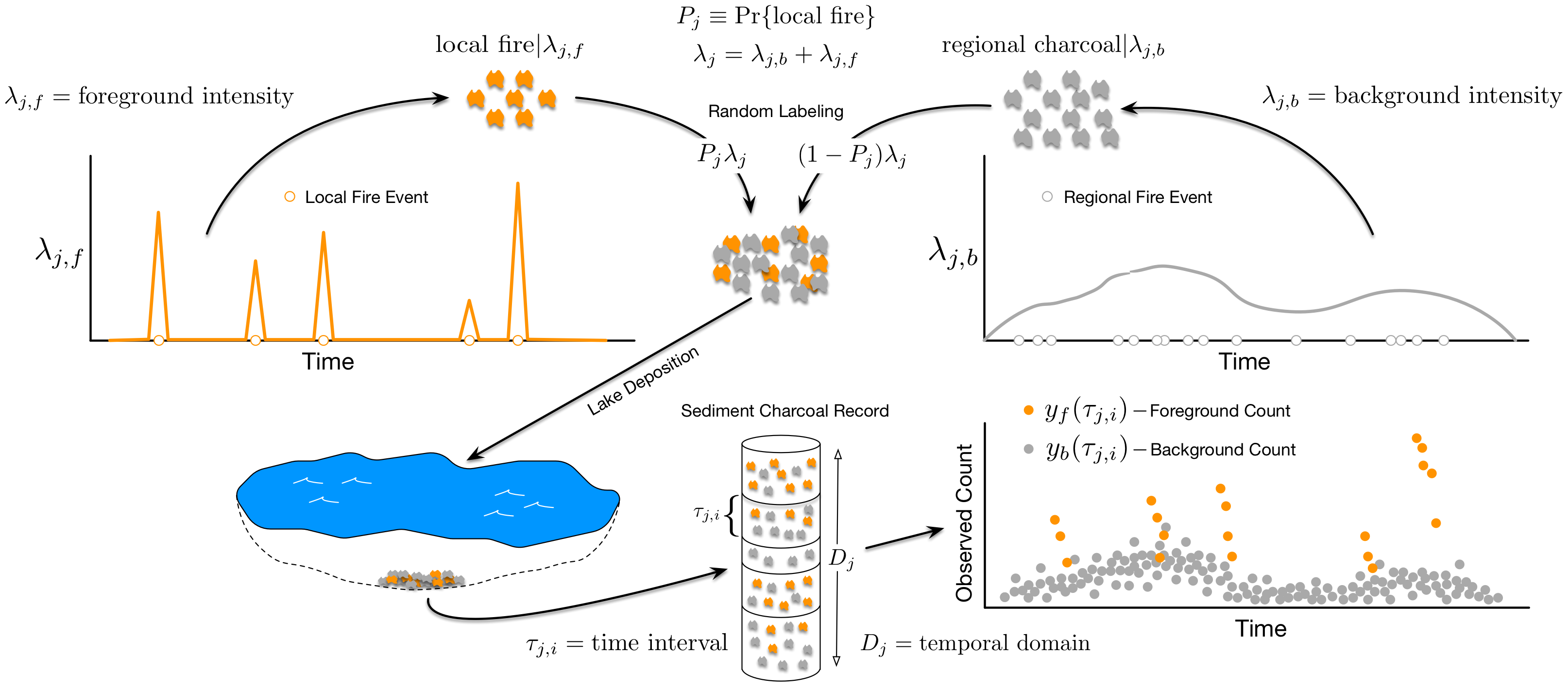
Figure 1: Illustration of theoretical charcoal deposition to a lake if charcoal particles arising from regional fires were distinguishable from particles arising from local fires (in practice, charcoal particles from different sources are indistinguishable). The figure does not depict charcoal arising from secondary sources such as surface water runoff or sediment mixing.

Figure 1 illustrates primary and regional charcoal deposition to a sample lake. We can think of charcoal deposition to a sample lake as being driven by two independent processes in time: a foreground process driving primary charcoal deposition during local fires, and a background process driving regional and secondary charcoal deposition. In practice, charcoal particles arising from different sources are indistinguishable in sediment charcoal records. We observe a single charcoal count over a fixed time interval. Direct estimation of foreground and background processes is not possible without separate background and foreground counts. We overcome the lack of explicit background and foreground counts by making strong assumptions about the nature of the background and foreground processes. Specifically, we assume the background process is smooth, exhibiting low-frequency changes over time, while the foreground process is highly-variable, exhibiting high-frequency changes in charcoal deposition rates associated with local fires. These assumptions follow directly from a long line of paleoecological research, which partitions charcoal into: 1) a background component that reflects regional charcoal production varying as a function of long-term climate and vegetation shifts; 2) a peak component reflecting local fire events and measurement error.

We use statistical regularization to ensure the assumption regarding the relative smoothness and volatility of the background and foreground processes is met. Under regularization, we seek the solution to an optimization problem (such as maximizing the likelihood of a parameter) subject to a constraint. The purpose of the constraint, in the context of Bayesian data analysis, is to bound the posterior distribution to some reasonable range. In this way, the constraint resembles an informative prior distribution. Additional details on statistical regularization can be found in Hobbs & Hooten (2015) and Hooten & Hobbs (2015).

In the context of sediment charcoal records, we model two deposition processes under the constraint that the background process is smooth, while the foreground process is volatile. We use unique sets of regression coefficients to model the background and foreground processes. Both sets of regression coefficients are assigned prior distributions, but with different prior variances. The prior variance for the foreground coefficients is much larger than the prior variance for the background coefficients. The prior variance parameters serve as the regulators (equivalent to a penalty term in Lasso or ridge regression) and force the background process to be smooth, while allowing the foreground process to be sufficiently flexible to capture charcoal deposition from local fires.

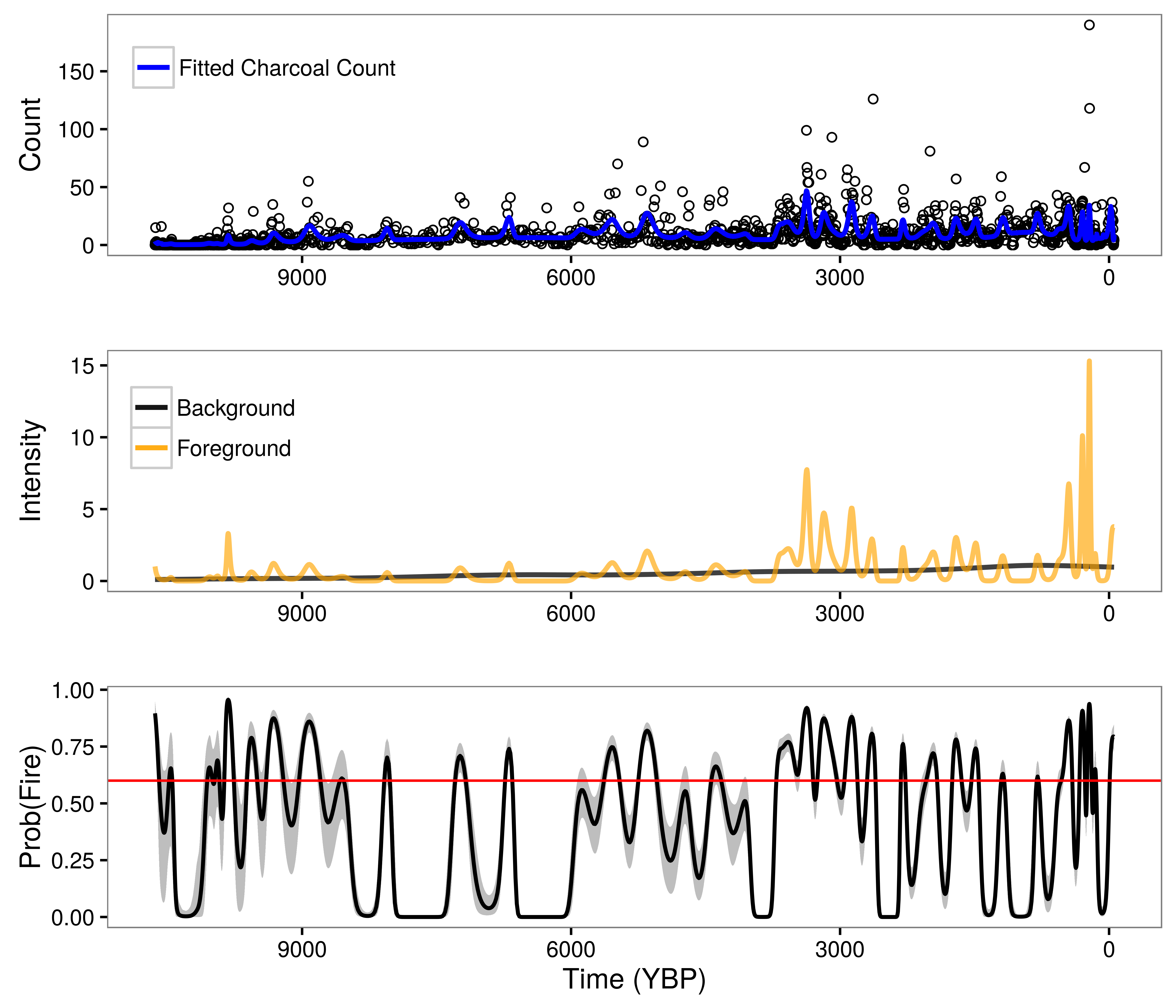
Figure 2: Model results for Screaming Lynx Lake, Alaska. Upper panel indicates observed charcoal counts along with the posterior mean charcoal count (blue line). Middle panel illustrates posterior mean foreground (orange line) and background (black line) deposition processes. Lower panel plots posterior mean probability of fire estimates for each observed time interval (black line) along with the upper and lower bounds of the 95 percent credible interval (gray shading) and an optimized local fire threshold (red line).

Figure 2 shows the results of regularization separation of background and foreground deposition processes from a single set of charcoal counts for Screaming Lynx Lake in Alaska. The probability of fire values presented in the lower panel of Figure 2 follow from the ratio of the foreground process relative to the sum of the background and foreground processes. We would not be able to identify the background and foreground processes without the strong assumption on the dynamics of the processes over time and the corresponding regularization. The benefits of using such an approach to model sediment charcoal deposition are: 1) our model reflects scientific understanding of charcoal deposition to lakes during and after fire events; 2) we are able to identify local fire events from noisy sediment charcoal records; 3) the background process provides a measure of regional fire dynamics, which can be correlated with climate and vegetation shifts over time.

References
1. Hobbs, N.T., Hooten, M.B. 2015. Bayesian Models: A Statistical Primer for Ecologists. Princeton University Press, Princeton, NJ.
2. Hooten, M.B., Hobbs, N.T. 2015. A guide to Bayesian model selection for ecologists. Ecololgical Monographs, 85, 3-28.
3. Itter, M.S., Finley A.O., Hooten, M.B., Higuera, P.E., Marlon, J.R., Kelly, R., McLachlan, J.S. (Submitted). A model-based approach to wildland fire reconstruction using sediment charcoal records. arXiv:1612.02382

State Data Assimilation and PalEON

Post by Michael Dietze and Ann Raiho

What is state data assimilation (SDA)?

SDA is the process of using observed data to update the internal STATE estimates of a model, as opposed to using data for validation or parameter calibration. The exact statistical methods vary, but generally this involves running models forward, stopping at times where data were observed, nudging the model back on track, and then restarting the model run (Figure 1). The approached being employed by the modeling teams in PalEON are all variations of ENSEMBLE based assimilation, meaning that in order to capture the uncertainty and variability in model predictions, during the analysis step (i.e. nudge) we update both the mean and the spread of the ensemble based on the uncertainties in both the model and the data. Importantly, we don’t just update the states that we observed, but we also update the other states in the model based on their covariances with the states that we do observe. For example, if we update composition based on pollen or NPP based on tree rings, we also update the carbon pools and land surface fluxes that co-vary with these.

Figure 1. Schematic of how state data assimilation works. From an initial state (shown as pink in the Forecast Step) you make a prediction (blue curve in the Analysis step). Then compare your data or new observation (green in the Analysis step) to the model prediction (blue) and calculate an updated state (pink in the Analysis step).

There are many components in the PalEON SDA and many people are involved. In all methods being employed by PalEON modeling teams, the uncertainty in the meteorological drivers is a major component of the model ensemble spread. Christy Rollinson has developed a workflow that generates an ensemble of ensembles of meteorological drivers – first she starts with an ensemble of different GCM’s that have completed the ‘last millennia’ run (850-1850 AD) and then downscales each GCM in space and time, generating an ensemble of different meteorological realizations for each GCM that propagates the downscaling uncertainty. John Tipton and Mevin Hooten then update this ensemble of ensembles, providing weights to each based on their fidelity with different paleoclimate proxies over different timescales. In addition to the meteorological realizations, some of the techniques being employed also accommodate model parameter error and model process error (which is like a ‘residual’ error after accounting for observation error in the data).

Why are we doing SDA in PalEON?

In the PalEON proposals we laid out four high-level PalEON objectives: Validation, Inference, Initialization, and Improvement. Our previous MIP (Model Intercomparison Project) activities at the site and regional scale were focuses specifically on the first of these, Validation. By contrast, SDA directly informs the next two (Inference, Initialization). Both the SDA and the MIP indirectly support the fourth (Improvement).

In terms of Inference, the central idea here is to formally fuse models and data to improve our ability to infer the structure, composition, and function of ecosystems on millennial timescales. Specifically, by leveraging the covariances between observed and unobserved states we’re hoping that models will help us better estimate what pre- and early-settlement were like, in particular for variables not directly related to our traditional paleo proxies (e.g. carbon pools, GPP, NEE, water fluxes, albedo). The last millennium is a particularly important period to infer as it’s the baseline against which we judge anthropogenic impacts, but we lack measurements for many key variables for that baseline period. We want to know how much we can reduce the uncertainty about that baseline.

In terms of Initialization, a key assumption in many modeling exercises (including all CMIP / IPCC projections) is that we can spin ecosystems up to a presettlement ‘steady state’ condition. Indeed, it is this assumption that’s responsible for there being far less model spread at 1850 than for the modern period, despite having far greater observations for the modern. However, no paleoecologist believes the world was at equilibrium prior to 1850. Our key question is “how much does that assumption matter?” Here we’re using data assimilation to force models to follow the non-equilibrium trajectories they actually followed and assessing how much impact that has on contemporary predictions.

Finally, SDA gives us a new perspective on model validation and improvement. In our initial validation activity, as well as all other MIPs and most other validation activities, if a model gets off to a wrong start, it will generally continue to perform poorly thereafter even if it correctly captures processes responsible for further change over time. Here, by continually putting the model back ‘on track’ we can better assess the ability of models to capture the system dynamics over specific, fixed time steps and when in time & space it makes reasonable vs unreasonable predictions.

SDA Example

Figure 2 shows a PalEON SDA example for a 30 year time period using tree ring estimates of aboveground biomass for four tree species from data collected at UNDERC and a forest gap model called LINKAGES.  The two plots show the tree ring data for hemlock and yellow birch in green, the model prediction in purple and the pink is how the data “nudge” the model. The correlation plot on the right represents the process error correlation matrix.  That is, it shows what correlations are either missing in LINKAGES or are over represented. For example, the negative correlations between hemlock vs. yellow birch and cedar suggest there’s a negative interaction between these species that is stronger than LINKAGES predicted, while at the same time yellow birch and cedar positively covary more than LINKAGES predicted. One interpretation of this is that hemlock is a better competitor in this stand, and yellow birch and cedar worse, than LINKAGES would have predicted. Similarly, the weak correlations of all other species with maple doesn’t imply that maples are not competing, but that the assumptions built into LINKAGES are already able to capture the interaction of this species with its neighbors.

Figure 2. SDA example of aboveground biomass in the LINKAGES gap model. The left and middle plots are the biomass values through time given the data (green), the model predictions (purple), and the updated model-data output (pink). The plot on the right is a correlation plot representing the process error correlation matrix.


Expert Elicitation to Interpret Pollen Data

Post by Andria Dawson, Post-Doc at the University of Arizona and the University of California-Berkeley

Fossil pollen counts from sediments collected from bogs, lakes, or forest hollows tell us something about the composition of surrounding forests (read more about fossil pollen here and here). In a sediment core, pollen samples from multiple depths tell us about changes in these surrounding forests over time. Barring some rare and complex geophysical events, going deeper means going back in time. With some simplifying assumptions about how pollen travels from tree to sediment we can use counts of sediment pollen grains to quantitatively reconstruct forests of the past.

However, correlating depth with time, or aging the sediment, is a difficult problem. Sediment accumulates at rates that vary through time, resulting in non-linear age-depth relationships. This means that knowing the sampling year – or the age of the surface sediment – is not enough to reliably estimate the ages of samples from further down in the sediment. This lack of information is solved with radiometric dating. Small pieces of plant material from the surrounding environment find their way into the sediment; these are macrofossils. Isotope signatures from these macrofossils can be used to determine their approximate age, and provide us with additional age-depth data points. Age-depth models can be constructed from these age-depth data points.

Another way to link depth with age is to look for signatory changes in pollen representation over time. Hallmark changes in the representation of indicator taxa allow scientists to associate sediment depths with events whose dates (ages) are roughly known. In the upper midwestern US, European settlement led to significant land-use changes which resulted in increases in several agricultural indicator taxa, including ambrosia (i.e., ragweed) and rumex (i.e., docks and sorrels) (Figure 1). This change in pollen representation makes it possible to identify pre- and post-settlement depths in a pollen sediment core. This matters because some scientists (including some of us on PalEON) hypothesize that major land-use changes probably caused big changes in the pollen-vegetation relationship. Were these anthropogenically-induced changes in the pollen-vegetation relationship greater than what we would expect without this external forcing? We don’t know, and might never know.

Images of A) ragweed and B) sheep sorrel.

Images of A) ragweed and B) sheep sorrel.

Nevertheless, we want to identify what we often refer to as the settlement horizon in the pollen records for at least two reasons. First, it allows us to compare pollen from the time of European settlement with public land survey records. Second, it is often used as an additional age-depth data point in the construction of age-depth models. But how easy is it to identify this settlement horizon? Recent work shows it is not as easy as one might have thought.

The unofficial PalEON mantra is that it is better to be correct and uncertain than certain and wrong. This line of thought led us to conduct an experiment using expert elicitation, where experts were tasked with identifying the settlement horizon in pollen records from the upper midwest. Four experts each considered 185 pollen records from the upper midwest USA. For 59 pollen records the experts agreed on the location of the settlement horizon (Figure 2). For the remaining records, there was some level of disagreement (Figure 3). This is not surprising, but does highlight the importance of thinking about uncertainty. Does this mean that we should disregard all previous attempts to identify the settlement horizon? The answer to this is a resounding no. The moral from all of this is that understanding your data is critical; understand its uncertainty and how this impacts your work. In the age of big-data and data-sharing, it becomes more difficult to really know your data, but the payoff is sound science. Know your data, and know it well.

To learn more about how we use results from the expert elicitation exercise referred to above, check out our recent Dawson et al. 2016 paper in Quaternary Science Reviews where we calibrate the pollen-vegetation relationship. Elicitation results have also been used to redefine controls for a new suite of age-depth models (Goring et al., in prep), which will in turn be used to assign dates to pollen samples used in vegetation reconstructions (Dawson et al, in prep).


Figure 2. Example of a pollen diagram from a site where experts were in complete agreement on the location of the representative pre-settlement sample. Samples identified by experts as pre-settlement are indicated by the dashed lines.

Figure 2. Example of a pollen diagram from a site where experts were in complete agreement on the location of the representative pre-settlement sample. Samples identified by experts as pre-settlement are indicated by the dashed lines.

Pollen Diagram Figure 3

Figure 3. Example of a pollen diagram from a site where experts were in complete disagreement on the location of the representative pre-settlement sample. Samples identified by experts as pre-settlement are indicated by the dashed lines.

References

  1. Dawson, Paciorek, McLachlan, Goring, Williams, Jackson. 2016. Quantifying pollen-vegetation relationships to reconstruct ancient forests using 19th-century forest composition and pollen data. Quaternary Science Reviews.137: 156-175. 
  2. Goring, Dawson, Grimm, et al. Semi-automated age model development for large scale databases. 2016. In prep for submission to Open Quaternary.
  3. Dawson, Paciorek, McLachlan, Goring, Williams, Jackson. 2016. Pre-industrial baseline variation of upper midwestern US vegetation. In prep for submission to Quaternary Science Reviews.

Reconstructing Multivariate Climate Using A Mechanistic Tree Ring Model

Post by John Tipton, statistics graduate student with Mevin Hooten at Colorado State University

Statistical Challenges of Paleoclimate Reconstructions
The ability to reconstruct paleoclimate from proxy data is important for understanding how climate has changed in the past and to allow exploration into how changing climate influences ecological processes. Statistical reconstructions of paleoclimate have unique challenges because proxy data are noisy, indirect observations of climate. Thus, any statistical model must address the following challenges: change of temporal support, sparse data, and the prediction of unobserved climate variables. When reconstructing climate from tree ring widths, the change of temporal support arises because our climate data are monthly average temperature and log total precipitation, whereas tree ring growth is measured on an annual scale. Therefore, any statistical model must account for this temporal misalignment. To overcome estimation issues common in sparse data scenarios, many previous reconstructions used linear statistical methods with constraints to regress the tree ring widths onto climate. For a multivariate climate reconstruction (e.g., temperature and precipitation), predicting paleoclimate using linear regression requires the inversion of a many to one functional that has potentially infinite solutions. Thus, multivariate climate reconstructions from univariate tree ring width time series are not commonly performed.

Mechanistic Models – A Promising Alternative
There is a need for rigorous statistical multivariate climate reconstructions, and hence, we developed an alternative to using linear statistical methods (Tipton et. al., In Press), using a mechanistic, biologically motivated model that “grows” tree rings to approximate the true growth process. By growing tree ring widths on a monthly time step, the mechanistic model aligns the monthly climate data with annual tree ring width data. Extending the mechanistic model to allow each tree species to have differential response to climate provides strong constraints on possible climate scenarios, ameliorating the difficulties that arise from having too many unknowns. We perform Bayesian inference to generate a probabilistic reconstruction that allows visual exploration of uncertainties. In contrast, many paleoclimate reconstructions generate point estimates that are not probabilistic in nature. The probabilistic reconstructions provide auxillary information that can be used to determine at what time periods the reconstruction is informative. Unfortunately, the use of a mechanistic growth model comes at a computational cost, thus we fit our model using Markov Chain Monte Carlo with compiled C++ code to increase computation speed.

Reconstruction of T and P – at the Same Time!
Our motivating goal was to generate a reconstruction of spatially explicit climate (temperature and precipitation) in the Northeastern United States that can be used to better understand how vegetation patterns have changed due to both climate change and direct human activity. Our work focuses on the Hudson Valley of New York, although in future work this model framework could be extended to the entire Northeastern United States. We focus on the Hudson Valley because there has been previous efforts to reconstruct the Palmer Drought Severity Index (PDSI), a combination of temperature and precipitation, which we can directly compare to our reconstruction, exploring the benefits and costs of different modeling frameworks. Figure 1 shows our joint temperature and precipitation reconstruction with the darkness of the shaded areas proportional to the probabilistic model predictions. For comparison, the black line in the log precipitation plot represents the previous centered and scaled PDSI reconstruction. Interestingly, there is little learning about temperature from our model (although the uncertainties are reasonable) while the log precipitation reconstruction is highly correlated (r=0.72) with the preexisting PDSI reconstruction. This result is in line with ecological expectations – drought in the Hudson Valley is strongly associated with precipitation (Pederson et al., 2015). When comparing our reconstruction to the previous efforts, our method has the added benefit of providing uncertainty estimates that illuminate where in time the reconstruction is informative without relying on statistically improper scoring rules like RE and CE commonly used in the paleoclimate literature. The use of proper scoring rules for assessing predictive ability is vital, because improper scoring rules can lead to incorrect inference about predictive skill.

Figure 1. Plot of probabilistic reconstruction of temperature and log precipitation using a mechanistic tree ring growth model. The reconstructions are shaded according to posterior predictive probabilities with the dotted lines giving the 95% credible interval. The solid black line in the log precipitation plot is a centered and scaled reconstruction of PDSI using the same data. The black lines at the far right of each reconstruction are the observational records.

Figure 1. Plot of probabilistic reconstruction of temperature and log precipitation using a mechanistic tree ring growth model. The reconstructions are shaded according to posterior predictive probabilities with the dotted lines giving the 95% credible interval. The solid black line in the log precipitation plot is a centered and scaled reconstruction of PDSI using the same data. The black lines at the far right of each reconstruction are the observational records.

What Did We Learn?
Reconstructing climate based on ecological proxies is tricky! Our simulations showed that the model we developed can reconstruct multivariate climate with great skill when tree growth responds to both temperature and precipitation. However, in the Hudson Valley, and many other temperate regions, trees respond mainly to precipitation and the bulk of tree growth occurs in a very limited range of temperatures. Thus, while the reconstruction of precipitation in these regions is both accurate and precise, the reconstruction of temperature is inherently more uncertain. The main benefit of a fully rigorous approach for obtaining the reconstructions is that the proper uncertainty can then be factored in to our scientific understanding of the climate process as well as accounted for in other modeling efforts (e.g., ecosystem computer models that depend on historic climate reconstructions).

References
Pederson, N., A.W. D’Amato, J.M. Dyer, D.R. Foster, D. Goldblum, J.L. Hart, A.E. Hessl, L.R. Iverson, S.T. Jackson, and D. Martin-Benito. (2015). Climate remains an important driver of post-European vegetation change in the eastern United States. Global Change Biology, 21(6), 2105-2110.

Tipton, J.R., M.B. Hooten, N. Pederson, M.P. Tingley, and D. Bishop. (In Press).
Reconstruction of late Holocene climate based on tree growth and mechanistic hierarchical models. Environmetrics.

Big process, small data: Reconstructing climate from historical U.S. fort data

Post by John Tipton, statistics graduate student with Mevin Hooten at Colorado State University, about work John and Mevin are doing with Jack Williams and Simon Goring.

Big data” has very rapidly become a popular topic. What are big data? The concept of big data in statistics is the analysis of very large datasets with the goal of obtaining inference in a reasonable time frame. The paleoclimate world often has the opposite problem: taking small amounts of data and expanding to produce a spatially and temporally rich result while accounting for uncertainty. How do you take a handful of temperature observations and predict a temperature surface over 20,000 locations for a period of 73 years in the past? Perhaps some of the techniques used in big data analysis can help.

Figure 1. Four representative years of temperature records (ºC) from the historical fort network.

Figure 1. Four representative years of temperature records (ºC) from the historical fort network.

The U.S. fort data consist of temperature records from military forts in the Upper Midwest region of the United States from 1820-1893. A subset of these instrumental temperature records (Figure 1) illustrates the sparse nature of the historical U.S. fort data relative to the spatial area of interest, especially in the earlier two years (1831 and 1847). From the small set of temperature observations collected each year, we seek to reconstruct average July temperature at a fine grid of 20,000 prediction locations. Techniques such as optimal spatial prediction, dimension reduction, and regularization allow us to provide formal statistical inference for this very large underlying process using a relatively small set of observational data.

To ameliorate the sparsity of the fort data, we used patterns from recent temperature fields (i.e., PRISM products) as a predictor variables in a Bayesian hierarchical empirical orthogonal function regression that includes a correlated spatial random effect. A strength of this modeling technique is that the primary patterns of temperature should remain stable even though the magnitude might change (e.g., it will always be cooler in the north than in the south). Another characteristic of this methodology is that it allows for localized differences in prediction to arise through a correlated spatial random effect. The correlated spatial random effect is too computationally expensive to calculate using traditional methods so the effect is estimated using big data techniques. Specifically, any remaining correlation that ties the fort locations together beyond that predicted by combinations of the primary temperature patterns is approximated in a lower dimensional space. This greatly reduces the computational effort needed to fit the model. We also employ a type of model selection technique called regularization to borrow strength from years with more data. This results in predictions that are close to the historical mean when there are few observations in a given year, while allowing for more detailed predictions in years with more data. To make the model selection computationally feasible, we fit the model in a highly parallelized high performance cluster computing environment.

The use of big data techniques for large paleoclimate reconstruction allows for statistical estimation of climate surfaces with spatially explicit uncertainties. Results of the mean July temperature for the subset of four years are shown in Figure 2, while the associated spatially explicit uncertainties are shown in Figure 3. These figures illustrate the strengths of the modeling techniques used. In the two earlier years, the predictions are similar to the historical mean with uncertainty increasing as a function of distance from observations. In the two later years with more data, the predictive surfaces have more spatial complexity and less associated uncertainty.

Figure 2. Reconstruction based on the posterior mean July temperature (ºC) for four representative years of the historical fort network.

Figure 2. Reconstruction based on the posterior mean July temperature (ºC) for four representative years of the historical fort network.

Figure 3. Posterior standard deviation surface of mean July temperature (ºC) for four representative years of the historical fort network.

Figure 3. Posterior standard deviation surface of mean July temperature (ºC) for four representative years of the historical fort network.

By explicitly accounting for latent correlated spatial structure and moderating model complexity using regularization, spatio-temporal predictions of paleoclimate are improved. Furthermore, dig data techniques allow us to fit the statistical models in a reasonable time frame (i.e., on the order of days rather than weeks). The relatively small sample sizes commonly associated with paleoclimate data would not normally fall into the “big data” realm of analyses. However, the processes on which we seek inference are quite large, and thus “big data” techniques are tremendously helpful.


Sneak Peek at Results for Tree Composition Pre-Euro-American Settlement (ca. 1700-1850 AD)

Posted by Jody Peters with input from Simon Goring and Chris Paciorek

Just as many trees make up a mighty forest, many participants are needed to pull together and analyze data for PalEON.  Together we gain a deeper understanding of past forest dynamics, and use this knowledge to improve long-term forecasting capabilities.  Major components needed to understand past forest dynamics are tree composition, density and biomass prior to Euro-American settlement. In true macrosystems ecology fashion, over the past 3 years (and in some cases longer) individuals from multiple institutions (see Table and Figure captions, and Figure 3 here) have been working on collecting the data and developing a statistical multinomial model for tree composition in the Northeast and Midwest United States.  Our first task has been to estimate percent composition for several of the dominant forest taxa, and to provide reliable estimates of uncertainty.

We are excited to announce we have finally collected enough data to run the model across the entire northeastern United States!  Figure 1 provides an example of the composition results and associated uncertainty for beech and pine.  In addition to these two genera we have similar results for taxa such as oak, birch, hickory, maple, spruce, etc.  We can use these results to compare the pre-European Settlement forest composition to modern forests from US Forest Service Forest Inventory Assessment data as well as those extending 2000 years into the past using pollen data and STEPPS2 analyses (see this University of Wisconsin Press Release).  As we move forward with this project we will continue to update our datasets that have dispersed sampling (e.g., Indiana, Illinois and Ohio: Table 1) and we are in the process of developing maps of estimated density and biomass by tree taxon.

Stay tuned as more results come in and as the manuscripts get published!


Figure 1. Estimated composition (top maps) and associated uncertainty (bottom maps) created March 2014. Estimates come from a spatial multinomial model on an 8 km Albers grid, developed by Andy Thurman from the University of Iowa and Chris Paciorek from the University of California, Berkeley. The MCMC was run for 150,000 iterations, with the first 25,000 discarded as burn-in, and the remaining iterations subsampled (to save on storage and computation) to give 500 posterior draws.

Figure 1. Estimated composition (top maps) and associated uncertainty (bottom maps) created March 2014. Estimates come from a spatial multinomial model on an 8 km Albers grid, developed by Andy Thurman from the University of Iowa and Chris Paciorek and Andria Dawson from the University of California, Berkeley. The MCMC was run for 150,000 iterations, with the first 25,000 discarded as burn-in, and the remaining iterations subsampled (to save on storage and computation) to give 500 posterior draws.
Click on the image for a bigger, clearer picture.


Table 1. Source of tree data from Public Land Surveys from locations in the Northeast and Midwest United States. The “Sampling” column indicates when data came from the entire location (complete) or from a dispersed sample of townships or towns within the location.

LocationSamplingSource
MinnesotaCompleteDavid Mladenoff(University of Wisconsin - Madison)
WisconsinCompleteDavid Mladenoff(University of Wisconsin - Madison)
Michigan's Upper Peninsula & northern Lower PeninsulaCompleteMichigan Department of Natural Resources; David Mladenoff
Michigan's southern Lower PeninsulaDispersedJack Williams & Simon Goring
(University of Wisconsin - Madison)
IllinoisDispersedJason McLachlan (University of Notre Dame)
Illinois Chicago areaCompleteMarlin Bowles & Jenny McBride (The Morton Arboretum)
Illinois St. Louis areaCompleteDick Brugam (Southern Illinois University) & Paul Kilburn (Jefferson County Nature Association)
IndianaDispersedJason McLachlan (University of Notre Dame)
OhioDispersedCharles Cogbill
New England, New Jersey, New York and PennsylvaniaDispersedCharles Cogbill

Self thin you must

yoda

Post by Dave Moore, Professor at The University of Arizona
This post also appeared on the Paleonproject Tumblr

We spent a lot of time last week in Tucson discussing sampling protocols for PalEON’s tree ring effort that will happen this summer. The trouble is that trees (like other plants) will self thin over time and when we collect tree cores to recreate aboveground biomass increment we have to be careful about how far back in time we push our claims. Bonus points if you can explain the photo in ecological terms! I stole it from Rachel Gallery’s Ecology class notes.

Neil Pederson and Amy Hessl will be taking the lead in the North East while Ross Alexander working with Dave Moore and Val Trouet (LTRR) will push our sampling into the Midwest and beyond the PalEON project domain westwards. This is a neat collaboration between the PalEON project and another project funded by the DOE. Francesc Montane and Yao Liu who recently joined my lab will be helping to integrate these data into the Community Land Model. Also Mike Dietze‘s group will be using the ED model to interpret the results.

Because we want to integrate these data into land surface models we need to have a robust statistical framework so we had some equally robust discussions about statistical considerations with Chris Paciorek and Jason McLachlan and other members of the PalEON team.