Pollen Dispersal I: Why We Get Sediment Pollen

Post by Andria Dawson, Post-Doc at University of California-Berkeley

Pollen and seed dispersal are important reproductive processes in plants, and in part determines the abundance and extent of a species. With a recent push to understand how species will respond to global climate change, dispersal ecology has gained increasing interest. We really want to know if there is a dispersal limitation, or if species can migrate quickly enough to maintain survival in a changing environment. Addressing this question presents challenges, many of which arise from trying to understand and quantify dispersal in ecosystems that are changing in both space and time (Robledo-Arnuncio 2014).
Pollen
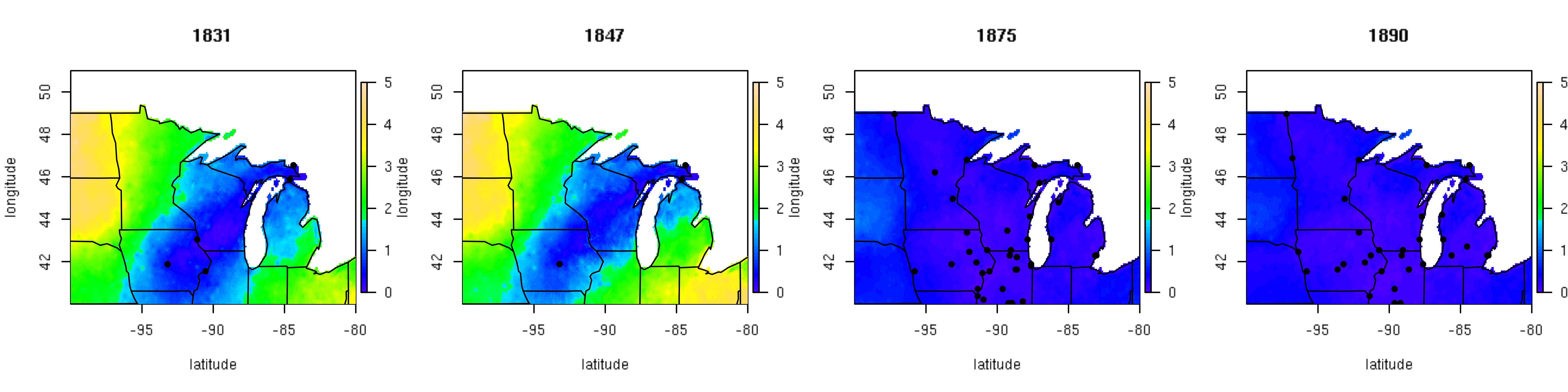
In PalEON, one of our efforts involves estimating the past relative abundance of vegetation from fossil pollen records. To do this, we need to quantify the pollen-vegetation relationship, which includes modelling pollen dispersal processes.

For many trees, including those we study in the PalEON domain, pollination is exclusively (or at least predominantly) anemophilous (carried out by wind). In angiosperms, wind pollination is thought to have evolved as an alternative means of reproduction for use when animal pollinators are scarce (Cox 1991). It was previously understood that wind pollination was less efficient than insect pollination (Ackerman 2000), but Friedman and Barrett (2009) show that may not be the case. To estimate the efficiency of wind pollination, they compared pollen captured by stigmas to pollen produced, and found that the mean pollen capture was about 0.32%, which is similar to estimates of animal pollination efficiency. Although both dispersal vectors are comparable with respect to efficiency, these quantities indicate that both are still pretty inefficient – this is great news for paleoecologists! Some of the pollen that is not captured ends up in the sediment.

Now we know that we expect to find pollen in the sediment, but how do we begin to quantify how much pollen of any type we expect to find at a given location? The route a pollen grain takes to arrive at its final location is governed by atmopsheric flow dynamics (among other things). These dynamics are complicated by landscape heterogeneity and climate, and differ among and within individuals because not all pollen grains are created equal. However, we usually aren’t as interested in the route as we are in the final location – in particular, we want to know the dispersal location relative to the source location. The distributions of dispersal locations from a source defines a dispersal kernel which can be empirically estimated with dispersal location data. Often these kernels are modelled using parametric distributions, usually isotropic, and often stationary with respect both space and time. Are these approximations adequate? If so, at what scale? These are some of the questions we hope to address by using Bayesian hierarchical modelling to quantify the pollen vegetation relationship in the Upper Midwest.

References
1. Robledo-Arnuncio, JJ, et al. Movement Ecology, 2014.
2. Cox, PA. Philosophical Transactions of the Royal Society B: Biological Sciences, 1991.
3. Friedman, J, Barrett SCH. Annals of Botany, 2009.
4. Ackerman, JD. Plant Systematics and Evolution, 2000.

Underwater In New England

Post by Bryan Shuman, Associate Professor of Geology & Geophysics at the University of Wyoming

To evaluate how forests have responded to climate change in the past, we need to reconstruct the climate history. Fortunately, in terms of moisture, lakes provide a geological gauge of precipitation (P) minus evapotranspiration (ET). As effective moisture (P-ET) changes, the water tables and lake surfaces rise and fall in elevation. When this happens, sands and other materials that typically accumulate near the shore of a lake are either moved deeper into the lake during low water or shift out from the lake’s center as water levels rise. Ongoing work in New England is building on existing datasets to provide a detailed picture of the multi-century trends in effective moisture. Here are a few highlights of recent progress.

First “the fun part” was fieldwork that I conducted while on sabbatical in New England. The work included a cold but fun day on the ice of Twin Pond in central Vermont with Laurie Grigg and students from Norwich University (pictured).

Coring at Twin Ponds

Coring at Twin Ponds

This trip was a follow up to a previous trip that coincided with Hurricane Sandy’s visit to New England in 2012. As the result of both trips, we now have a series of three cores that record shoreline fluctuations at the pond. Because the sediment contains both carbonate minerals and organic compounds, we have also been able to examine the ratios of oxygen and hydrogen isotopes in the sediment and provide some constraints on the temperature history too.

Ice makes coring easy (its stable), but the swimming was not as good as in the summer when I worked in southern New England with Wyatt Oswald (Emerson College), Elaine Doughty (Harvard Forest), and one of Harvard Forest’s REU students, Maria Orbay-Cerrato. Over several days, we collected new cores that record the Holocene water-level changes at West Side Pond in Goshen, Connecticut, and Green Pond, near Montague, Massachusetts. Floating on a pair of canoes, we enjoyed the early summer sun, told jokes, ate delightful snacks brought from home by Wyatt, and strained our muscles to pull about 5 cores out of each lake. Near shore, the cores from both lakes contained alternating layers of sand and mud consistent with fluctuating water levels. In the lake center at West Side Pond, we also obtained two overlapping cores about 14 m long, which promise to provide a detailed pollen record. Both lakes proved to be excellent swimming holes too!

Second, on a more earnest note, the existing geological records of lake-level change from Massachusetts have been synthesized in a recent (2014) paper in Geophysical Research Letters by Paige Newby et al. The figure shown here summarizes the results and compares the reconstructions with the pollen-inferred deviation from modern annual precipitation levels from a paper by University of Wyoming graduate student, Jeremiah Marsicek, last year (2013) in Quaternary Science Reviews.

Figure 4 from Newby et al. 2014

Figure 4 from Newby et al. 2014

All of the records show a long-term rise in effective moisture since >7000 years ago as well as meaningful multi-century deviations. By accounting for the age uncertainties from the reconstructions, we were able to show that a series of 100-800 year long droughts at 4200-3900, 2900-2100, and 1300-1200 years before AD 1950 affected lake levels (blue curves with reconstruction uncertainty shown) on Cape Cod (Deep Pond), the coastal Plymouth area (New Long Pond), and the inland Berkshire Hills (Davis Pond) – as well as the forest composition as recorded by the pollen from Deep Pond (red line). Interestingly, an earlier drought in the Berkshires at 5700-4900 years ago was out of phase with high water recorded in the eastern lakes. This difference is one of the motivations for the new work in Vermont, Connecticut and central Massachusetts, as well as other ongoing work with Connor Nolan in central Maine: what are the spatial patterns of drought?

Big process, small data: Reconstructing climate from historical U.S. fort data

Post by John Tipton, statistics graduate student with Mevin Hooten at Colorado State University, about work John and Mevin are doing with Jack Williams and Simon Goring.

Big data” has very rapidly become a popular topic. What are big data? The concept of big data in statistics is the analysis of very large datasets with the goal of obtaining inference in a reasonable time frame. The paleoclimate world often has the opposite problem: taking small amounts of data and expanding to produce a spatially and temporally rich result while accounting for uncertainty. How do you take a handful of temperature observations and predict a temperature surface over 20,000 locations for a period of 73 years in the past? Perhaps some of the techniques used in big data analysis can help.

Figure 1. Four representative years of temperature records (ºC) from the historical fort network.

Figure 1. Four representative years of temperature records (ºC) from the historical fort network.

The U.S. fort data consist of temperature records from military forts in the Upper Midwest region of the United States from 1820-1893. A subset of these instrumental temperature records (Figure 1) illustrates the sparse nature of the historical U.S. fort data relative to the spatial area of interest, especially in the earlier two years (1831 and 1847). From the small set of temperature observations collected each year, we seek to reconstruct average July temperature at a fine grid of 20,000 prediction locations. Techniques such as optimal spatial prediction, dimension reduction, and regularization allow us to provide formal statistical inference for this very large underlying process using a relatively small set of observational data.

To ameliorate the sparsity of the fort data, we used patterns from recent temperature fields (i.e., PRISM products) as a predictor variables in a Bayesian hierarchical empirical orthogonal function regression that includes a correlated spatial random effect. A strength of this modeling technique is that the primary patterns of temperature should remain stable even though the magnitude might change (e.g., it will always be cooler in the north than in the south). Another characteristic of this methodology is that it allows for localized differences in prediction to arise through a correlated spatial random effect. The correlated spatial random effect is too computationally expensive to calculate using traditional methods so the effect is estimated using big data techniques. Specifically, any remaining correlation that ties the fort locations together beyond that predicted by combinations of the primary temperature patterns is approximated in a lower dimensional space. This greatly reduces the computational effort needed to fit the model. We also employ a type of model selection technique called regularization to borrow strength from years with more data. This results in predictions that are close to the historical mean when there are few observations in a given year, while allowing for more detailed predictions in years with more data. To make the model selection computationally feasible, we fit the model in a highly parallelized high performance cluster computing environment.

The use of big data techniques for large paleoclimate reconstruction allows for statistical estimation of climate surfaces with spatially explicit uncertainties. Results of the mean July temperature for the subset of four years are shown in Figure 2, while the associated spatially explicit uncertainties are shown in Figure 3. These figures illustrate the strengths of the modeling techniques used. In the two earlier years, the predictions are similar to the historical mean with uncertainty increasing as a function of distance from observations. In the two later years with more data, the predictive surfaces have more spatial complexity and less associated uncertainty.

Figure 2. Reconstruction based on the posterior mean July temperature (ºC) for four representative years of the historical fort network.

Figure 2. Reconstruction based on the posterior mean July temperature (ºC) for four representative years of the historical fort network.

Figure 3. Posterior standard deviation surface of mean July temperature (ºC) for four representative years of the historical fort network.

Figure 3. Posterior standard deviation surface of mean July temperature (ºC) for four representative years of the historical fort network.

By explicitly accounting for latent correlated spatial structure and moderating model complexity using regularization, spatio-temporal predictions of paleoclimate are improved. Furthermore, dig data techniques allow us to fit the statistical models in a reasonable time frame (i.e., on the order of days rather than weeks). The relatively small sample sizes commonly associated with paleoclimate data would not normally fall into the “big data” realm of analyses. However, the processes on which we seek inference are quite large, and thus “big data” techniques are tremendously helpful.


Quaternary Science . . . on Mars . . . three billion years ago.

Post by Simon Goring, Research Assistant at the University of Wisconsin, Madison
Originally posted on OpenQuaternary Discussions.

For a curious person, one of the great benefits of being a Quaternary researcher is the breadth of research that is relevant to your own research questions.  The recent publication of fifty key questions in paleoecology (Seddon et al., 2014) reflects this breadth, spanning a broad range questions that reflect human needs, biogeophysical processes, ecological processes and a broad range of other issues.  The editorial board of Open Quaternary also reflects this incredible disciplinary breadth.  To me it is clear that the Quaternary sciences is an amalgam of multiple disciplines, and, at the same time, a broadly interdisciplinary pursuit.  To be successful one must maintain deep disciplinary knowledge in a core topic, as well as disciplinary breadth across topics such as ecology, anthropology, geology (and specifically geochronology), and you need a good grounding in statistics and climatology.

One of the things that is not always quite as apparent is the breadth of research affected by the Quaternary sciences.  My first exposure to the utility of paleoecology for understanding interplanetary dynamics came as the result of a paper we published two years ago.  In 2012, my co-authors and I developed a regional scale estimate of sediment deposition times in lakes across eastern North America for the Holocene (Goring et al, 2012). We did this because we were looking toward re-building age models for all cores in eastern North America and wanted to use reliable priors for Bacon (Blaauw and Christen, 2011).  Our priors wound up becoming the default in Bacon, which is great, but the results have also helped inform the lacustrine history of the red planet, Mars.


Figure 1. Paleo-lake level reconstruction in the Melas Baisn of Mars. From Williams and Weitz (2014).

Williams and Weitz (2014) were examining the Melas Basin, a feature of the Martian surface that appears to show evidence of lacustrine activity at some time in the past. Given a set of lacustrine features and channel beds in the basin, they began the process of trying to reconstruct lacustrine activity on the surface of Mars. It seems clear that if our own understanding of geophysical processes during the Quaternary is based on Whewell and Lyell’s concept of Uniformitarianism, that uniformity of process should not be limited to earth.

While we might assume uniformity, there are limits to how much modern or paleo terrestrial analysis can be applied to the Martian surface. Although the basin age is dated roughly using meteor strikes, the dating of lacustrine establishment and termination are much more difficult. For one, Holocene models rely on 14C dates. While it may be possible to obtain some form of geochronological information from the Martian surface, at some point it likely requires dating techniques we don’t have on hand.  However, researchers can develop experimental procedures to test the possibility of using other dating techniques, and it seems like development of these techniques is already underway with K-Ar dating (Hurowitz et al., 2012, PDF).

Another limitation of using Quaternary analysis is that our Holocene estimates rely on the assumption that there is near-modern vegetation cover, that sediment transport and flow rates are similar to modern and the distribution and types of sediment are similar to modern. Even in this assumption we know there are exceptions. Sediments deposited immediately following deglaciation are often very fine grained, we often see strong increases in organic content during the Holocene, and the presence of a major inflection point in deposition rates is a persistent feature of the near-modern era.

Regardless, to understand how long a lake was present in the Melas Basin there are few options but to look at earth systems. The Williams and Weitz paper (2014) looked at both deltaic sediments and lake sediments in the basin. Williams and Weitz (2014) estimate lacustrine activity using sedimentation rates from large deltas in the United States and Russia and our sedimentation rates for lacustrine environments. Interestingly, the deltaic sedimentation and lacustrine sedimentation rates seem off by orders of magnitude. In Goring et al. (2012) we show a mean sedimentation rate of approximately 20yr/cm, meaning the lacustrine environments of the Melas Basin might have persisted for almost 90,000 years, while sedimentation rates from the deltas produce estimates of between 1,000 and 4,000 years.

In a Holocene or Quaternary context, orders of magnitude between 1,000 and 100,000 seem incredibly broad. But, when we consider that we are examining the surface of another planet, and that the lake formation dates to the Hesperian period almost 3 billion years ago, the temporal certainty that Quaternary science can provide for interplanetary research is in fact astounding.

References Cited:

Blaauw, M, & Christen, JA (2011). Flexible paleoclimate age-depth models using an autoregressive gamma process. Bayesian Analysis6(3), 457-474.

Hurowitz, JA, et al. (2012). A New Approach to In-Situ K-Ar Geochronology. LPI Contributions, 1683, 1146.

Goring, S, et al. (2012). Deposition times in the northeastern United States during the Holocene: establishing valid priors for Bayesian age models.Quaternary Science Reviews,48, 54-60.

Seddon, AW, et al. (2014). Looking forward through the past: identification of 50 priority research questions in palaeoecology. Journal of Ecology102(1), 256-267.

Maine Fieldwork Part 2: The Bog

Post by Bob Booth, Associate Professor at Lehigh University; Steve Jackson, Center Director for the U.S. Department of the Interior’s Southwest Climate Science Center; Connor Nolan, Steve’s PhD Student at University of Arizona, and Melissa Berke, Assistant Professor at University of Notre Dame

Read about Maine Fieldwork Part 1.

Maine Fieldwork Part 2
Our adventures in bog coring, lobster consumption, dehydration, lake scouting, dipteran-slapping, and driving (lots of driving) began on July 6 when Bob Booth, Steve Jackson, Melissa Berke, and Connor Nolan rendezvoused in Portland, Maine, and drove to Bangor, our home base for coring at Caribou Bog. A testate-amoeba record of water-table depth from the bog will be compared to a lake-level record from Giles Pond (cored by Connor and Bryan Shuman back in November). These two sites are the new paleoclimate proxies for our Howland Forest HIPS (Highly Integrated Proxy Site). We also plan to use these records to better understand how lakes and peatlands respond to and record climate variation.

bog CaribouMap

Caribou Bog is a huge (~2200 hectares) ombrotrophic bog that has been the subject of many past investigations. We targeted a part of the bog that had been worked on in the 1980s by Feng Sheng Hu and Ron Davis. Coring took two full days (check out the video below to really appreciate the dipterans and the team’s jumping abilities). On the first day, we surveyed the bog with probbog - MBe rods to select a coring site. Then we hauled all of the heavy coring gear from the car, down a logging trail into the forest, through the “moat”, and then across the lumpy bog. Every part of the walk from the van to the bog and back was challenging, each for different reasons. The trail was hot and infested with deerflies and mosquitoes, the forest had no trail and low clearance and forced us to wrestle with young trees, the moat provided ample opportunity for losing boots and called for some gymnastic moves while carrying large and heavy stuff, and finally walking the 300 meters across the bog was like being on a demented stairmaster as we sunk a foot or two into the bog with every step.

bog flower - MB
After three trips to haul all of our gear, we cored the bog, collecting the upper peat (~3-4 meters) with a modified piston corer and the overlaps and deeper sections with a Russian corer. Although we thought we had ample drinking water the first day, we didn’t, and we chose not to drink the brown bog-water. Once we returned to the van, we headed straight to the nearest rural convenience store (only 3 miles away) and restored electrolytes and fluids.

We completed the coring on the second day, and dragged everything back to the van in three trips.  After dropping Bob off to meet his family in Portland, the rest of us enjoyed a seafood extravaganza at Fore Street restaurant in downtown Portland.  

portland head light

Portland Head Light

Lobster Feast

Lobster Feast

The cores went to Lehigh with Bob, but will eventually be analyzed by Connor. We will count testate amoebae and pollen in the core to get records of paleohydrology and paleovegetation spanning the past 2000 years.  Stay tuned!

Watch on YouTube: Caribou Bog 2014


Hu, F. S., & Davis, R. B. (1995). Postglacial development of a Maine bog and paleoenvironmental implications. Canadian Journal of Botany, 73(4), 638–649.


You Are Suffering For the Greater Good of Science

Post by Simon Goring, Postdoc at the University of Wisconsin-Madison.
This post originally appeared on downwithtime.

When you have hayfever you are suffering for the greater good of science.”
-Me. The Larry Meiller Show, WPR. July 16, 2014 [Program Archive]

Figure 1. Your pain is science's gain. Pollen may go into your nose, but it also enters aquatic environments where it is preserved in lake sediments. Photo Credit: flickr/missrogue

Figure 1. Your pain is science’s gain. Pollen may go into your nose, but it also enters aquatic environments where it is preserved in lake sediments. Photo Credit: flickr/missrogue

Of course, I was talking paleoecology and the way we use airborne pollen trapped in lake sediments to help improve models of future climate change. We improve models by reconstructing forests of the past. This is one of the central concepts in PalEON (not suffering, paleoecology): Improve ecosystem model predictions for the future by testing them on independent reconstructions of the past. Give greater weight to models that perform well, and improve models that perform poorly.

I was lucky to be on the Larry Meiller Show along with Paul Hanson to discuss PalEON and GLEON, two large scale ecological projects with strong links to The University of Wisconsin. We talked a bit about climate change, large scale research, science funding, open science and historical Wisconsin. It was lots of fun and you can check out the archive here.

I feel like I was a little more prepared for this interview than I have been in the past. Jack Williams passed along his (autographed) copy of Escape from the Ivory Tower by Nancy Baron. The book helped me map out my “message box” and gave me a much better sense of what people might want to hear, as opposed to the things I wanted to talk about (how much can I talk about uncertainty, age modelling and temporal connectivity?). It was useful, and I hope I came off as well prepared and excited by my research (because I am). Regardless, just like learning R, public outreach is a skill, and one that I am happy to practice, if only because I intend to keep doing it.

Anyway, enough science outreach for one week. With this blog post and WPR I’m well above quota!

Sneak Peek at Results for Tree Composition Pre-Euro-American Settlement (ca. 1700-1850 AD)

Posted by Jody Peters with input from Simon Goring and Chris Paciorek

Just as many trees make up a mighty forest, many participants are needed to pull together and analyze data for PalEON.  Together we gain a deeper understanding of past forest dynamics, and use this knowledge to improve long-term forecasting capabilities.  Major components needed to understand past forest dynamics are tree composition, density and biomass prior to Euro-American settlement. In true macrosystems ecology fashion, over the past 3 years (and in some cases longer) individuals from multiple institutions (see Table and Figure captions, and Figure 3 here) have been working on collecting the data and developing a statistical multinomial model for tree composition in the Northeast and Midwest United States.  Our first task has been to estimate percent composition for several of the dominant forest taxa, and to provide reliable estimates of uncertainty.

We are excited to announce we have finally collected enough data to run the model across the entire northeastern United States!  Figure 1 provides an example of the composition results and associated uncertainty for beech and pine.  In addition to these two genera we have similar results for taxa such as oak, birch, hickory, maple, spruce, etc.  We can use these results to compare the pre-European Settlement forest composition to modern forests from US Forest Service Forest Inventory Assessment data as well as those extending 2000 years into the past using pollen data and STEPPS2 analyses (see this University of Wisconsin Press Release).  As we move forward with this project we will continue to update our datasets that have dispersed sampling (e.g., Indiana, Illinois and Ohio: Table 1) and we are in the process of developing maps of estimated density and biomass by tree taxon.

Stay tuned as more results come in and as the manuscripts get published!


Figure 1. Estimated composition (top maps) and associated uncertainty (bottom maps) created March 2014. Estimates come from a spatial multinomial model on an 8 km Albers grid, developed by Andy Thurman from the University of Iowa and Chris Paciorek from the University of California, Berkeley. The MCMC was run for 150,000 iterations, with the first 25,000 discarded as burn-in, and the remaining iterations subsampled (to save on storage and computation) to give 500 posterior draws.

Figure 1. Estimated composition (top maps) and associated uncertainty (bottom maps) created March 2014. Estimates come from a spatial multinomial model on an 8 km Albers grid, developed by Andy Thurman from the University of Iowa and Chris Paciorek and Andria Dawson from the University of California, Berkeley. The MCMC was run for 150,000 iterations, with the first 25,000 discarded as burn-in, and the remaining iterations subsampled (to save on storage and computation) to give 500 posterior draws.
Click on the image for a bigger, clearer picture.


Table 1. Source of tree data from Public Land Surveys from locations in the Northeast and Midwest United States. The “Sampling” column indicates when data came from the entire location (complete) or from a dispersed sample of townships or towns within the location.

LocationSamplingSource
MinnesotaCompleteDavid Mladenoff(University of Wisconsin - Madison)
WisconsinCompleteDavid Mladenoff(University of Wisconsin - Madison)
Michigan's Upper Peninsula & northern Lower PeninsulaCompleteMichigan Department of Natural Resources; David Mladenoff
Michigan's southern Lower PeninsulaDispersedJack Williams & Simon Goring
(University of Wisconsin - Madison)
IllinoisDispersedJason McLachlan (University of Notre Dame)
Illinois Chicago areaCompleteMarlin Bowles & Jenny McBride (The Morton Arboretum)
Illinois St. Louis areaCompleteDick Brugam (Southern Illinois University) & Paul Kilburn (Jefferson County Nature Association)
IndianaDispersedJason McLachlan (University of Notre Dame)
OhioDispersedCharles Cogbill
New England, New Jersey, New York and PennsylvaniaDispersedCharles Cogbill

PalEON on TV

Posted by Jody Peters, PalEON Program Manager

The elevator pitch (a 30 second to 2 min synopsis of your research) is critical for sharing science with other scientists and the general public. However, developing this pitch usually does not come naturally to most people. It is something that needs to be practiced. Recently Jason McLachlan and Sam Pecararo from the University of Notre Dame, had the opportunity to practice their pitches in featured segments on Outdoor Elements, a show on our local PBS station. Not only did Jason and Sam have to prepare their elevator pitch, but they also had to come up with visual props that would be interesting to view on TV.  We think they both did a great job condensing their science stories into a few minutes!

Jason’s segment, Paleobotany & Climate Change, originally aired on Feb 9, 2014 and focused on PalEON in general and specifically described some of our work with tree data from the Public Land Survey. After he was taped for this segment last fall, Jason wrote a blog post about what he wished he would have said. Compare what he wished he would have said to what actually was aired!

JasonOutdoorElements

Sam’s segment, Tree Coring, originally aired on February 16, 2014 and featured Sam coring a tree and talking about using tree rings to get an idea of how climate or other environmental variables influence tree growth.

SamOutdoorElements

Check out these segments to see Jason and Sam’s elevator pitch for some of the work of PalEON! Click on the links or photos above and scroll down to where it says “Play segment” to view. Each segment is approximately 7 minutes long.


Self thin you must

yoda

Post by Dave Moore, Professor at The University of Arizona
This post also appeared on the Paleonproject Tumblr

We spent a lot of time last week in Tucson discussing sampling protocols for PalEON’s tree ring effort that will happen this summer. The trouble is that trees (like other plants) will self thin over time and when we collect tree cores to recreate aboveground biomass increment we have to be careful about how far back in time we push our claims. Bonus points if you can explain the photo in ecological terms! I stole it from Rachel Gallery’s Ecology class notes.

Neil Pederson and Amy Hessl will be taking the lead in the North East while Ross Alexander working with Dave Moore and Val Trouet (LTRR) will push our sampling into the Midwest and beyond the PalEON project domain westwards. This is a neat collaboration between the PalEON project and another project funded by the DOE. Francesc Montane and Yao Liu who recently joined my lab will be helping to integrate these data into the Community Land Model. Also Mike Dietze‘s group will be using the ED model to interpret the results.

Because we want to integrate these data into land surface models we need to have a robust statistical framework so we had some equally robust discussions about statistical considerations with Chris Paciorek and Jason McLachlan and other members of the PalEON team.

The Invasion of the Zombie Maples

Post by Ana Camila Gonzalez, Undergraduate Researcher with Neil Pederson and the Tree Ring Laboratory at Columbia’s Lamont-Doherty Earth Observatory

As an undergraduate student interning at the Tree Ring Lab at Lamont-Doherty Earth Observatory, my involvement with PalEON has been rather localized to the data production side of things. My knowledge on the dynamics of climate and the models involved in forecasting future climate change is obviously limited as a second-year student. My knowledge on how frustrating it can be to cross-date the rings in Maple trees, however, is more extensive.

This past summer I was able to join the Tree Ring Lab on a fieldwork trip to Harvard Forest in Petersham, MA. My main task was to map each plot where we cored, recording the species of each tree cored, its distance to the plot center, its DBH, its canopy position, its compass orientation, and any defining characteristics (the tree was rotten, hollow, had two stems, etc.). The forest was beautiful, but it became more beautiful every time I wrote down the letters QURU (Quercus rubra)I had plenty of experience with oaks, and knew that they did not often create false or missing rings and are thus a fairly easy species to cross-date. I shuddered a little every time I had to write down BEAL (Betula alleghaniensis), however, since I had looked at a few yellow birches before and knew the rings were sometimes impossible to see let alone cross-date. I had no reaction to the letters ACRU (Acer rubrum), however, since I had never looked at a red maple core before. I was happy that it was a tree I could easily identify, and so I didn’t mind that the letters kept coming up. Had I known what was to come, I would’ve found a way to prevent anyone from putting a borer to a red maple.

At first, the maples seemed to be my friends. The rings were sensitive enough that multiple marker years helped me figure out where the missing rings where, what was false and what was real. I morbidly became a fan of the gypsy moth outbreak of 1981, because in many cases (but not all) it produced a distinct white ring that marked that year very clearly. This was definitely challenging, as the trees also seemed to be locally sensitive (a narrow ring in one tree might not at all be present in another) but all in all it seemed to be going well.

And then came the Zombie Maples.

Fig (a) Anatomy of a White Ring: Above is a core collected in 2003. It was alive. The white ring in the center of the image is 1981, the year of the regional gypsy moth outbreak in New York and New England.

That white ring you’re seeing above is the characteristic 1981 ring from a Zombie Maple cored in 2003. After that ring we can only see four rings – but this tree is alive, which means that there should be 13 rings after 1990 (Fig b). This means approximately 10 are missing.

Fig (b) Anatomy of a Zombie Maple: Above is a core collected in 2003. It was alive. The 1990 ring is marked in the image just right of center. There should be 13 rings between 1990 and the bark. You can only see four. Is it Alive? Is it Dead? Eek! It is a Zombie!!

This kind of suppression in the last two decades was present in multiple cores, and it made many perfectly alive trees seem like they should have been dead. Nine rings missing in a little over one millimeter. We see even more severe cases in our new collection: 15 rings where there should be 30 rings in about 2 millimeters – how is this tree supporting itself?

Cross-dating these cores took a lot longer than planned, and at times I was tempted to pretend my box of maples went missing, but afterwards I felt I was a much stronger cross-dater, and I’m realizing more and more that this really matters. If you’re going to base a model off of data that involves ring-width measurements from particular years, you better make sure you have the right years. What if we didn’t know the gypsy moth outbreak occurred in 1981, and somebody counting the rings back on the Zombie maple core above was led to believe it occurred in 1996? Our understanding of the trigger for this event would be incorrect because we would be looking for evidence from the wrong decade.

In a way, the Maples are still my friends. They were almost like the English teacher in high school who graded harshly who you didn’t appreciate until you realized how much better your writing had become.