Models Part 1: The PalEON Model Inter-Comparison Project Comes to Life

Post by Christine Rollinson, Post-doc at Boston University working with Michael Dietze.

While writing what was intended as a single post about ecological modeling and PalEON, I discovered I had a lot more to say on the topic than I initially thought.  In the past year, I have moved from being an ecologist who spends every summer in the field (at a minimum) to one now mired in the world of models and computation.  I now see myself as something of a modeling ambassador whose goal it is to demystify the modeling process and increase communication and collaboration between the modeling and field-based ecologists.

This post is the first in a series on the ecological modeling side of PalEON and will focus on describing modeling in general and how it fits into the PalEON goals. Subsequent posts will discuss the modeling process in greater detail and how scientists like myself use these models to answer fundamental ecological questions.

ModelFig1

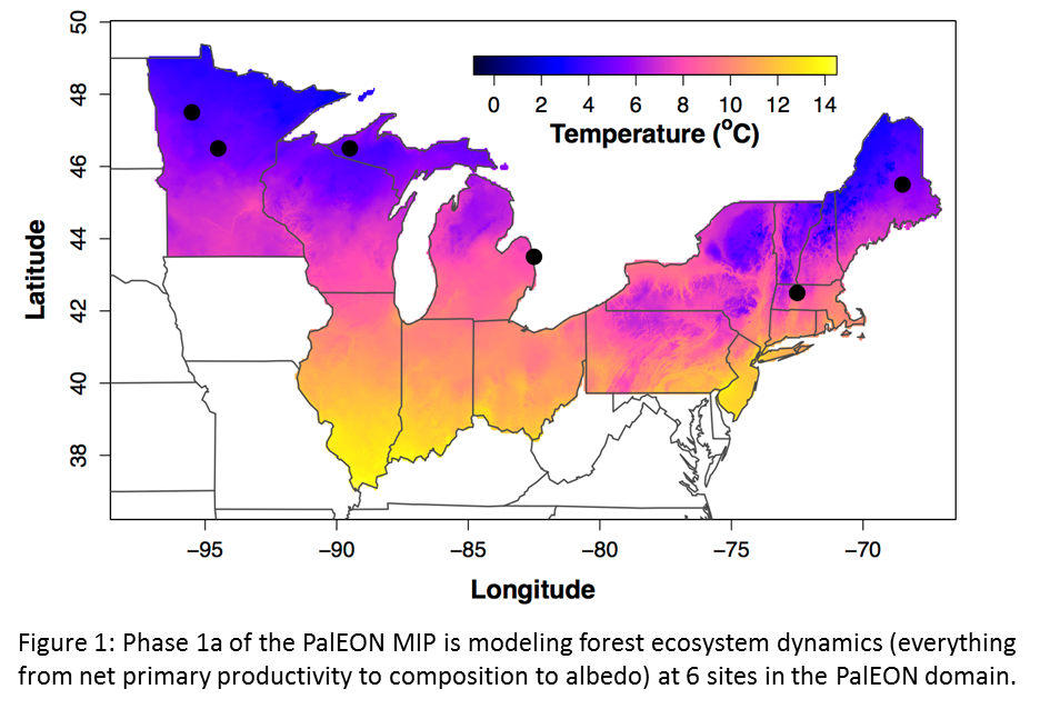
PalEON is collecting and synthesizing data from an incredible array of sources including tree rings, pollen, and historical records.  Although we have taken great care to geographically co-locate as much data collection as possible, these data contain information about very different aspects of ecosystems and at very different points in time. How can we combine information on centennial-scale changes in species composition from pollen records with sub-minute carbon fluxes from flux towers?  The answer is through models.

Before joining the PalEON modeling team, I, like many other field ecologists, assumed that because terrestrial ecosystem models have been used for a few decades now, the MIP (Model Inter-comparison Project) would merely be a matter of plugging in some meteorology drivers and then analyzing surprises in the output.  Oh how wrong I was!

Ecological Modeling 101
Whether we think about it or not, almost all scientists use models in one form or another.  The ANOVAs and simple linear regressions we use to statistically analyze our data are models. The terrestrial ecosystem models being used by the PalEON modeling group are essentially dozens, or sometimes hundreds, of these simple models combined.  Ecosystem modelers think about these complex models as scaffolds that let us relate physiological mechanisms for change (such as photosynthetic response to temperature) to coarser long-term patterns (such as changes in plant community composition).

As any ecologist will readily tell you, there is a lot about ecosystems that we don’t fully understand yet.  There are certain physiological processes such as photosynthesis and respiration that act as building blocks that form the foundation for how terrestrial plant ecosystems function.  However, there are still competing methods of characterizing those various building blocks and linking them together.  These different representations of how ecosystems function have led to the creation of multiple ecosystem simulation models¹.  Rather than limit itself to a single model and theory of how ecosystems function, PalEON is working with an international group of researchers to explore how as many models as possible predict ecosystem change to past environmental variability.

Modeling Past Ecosystem ChangeModelFig2

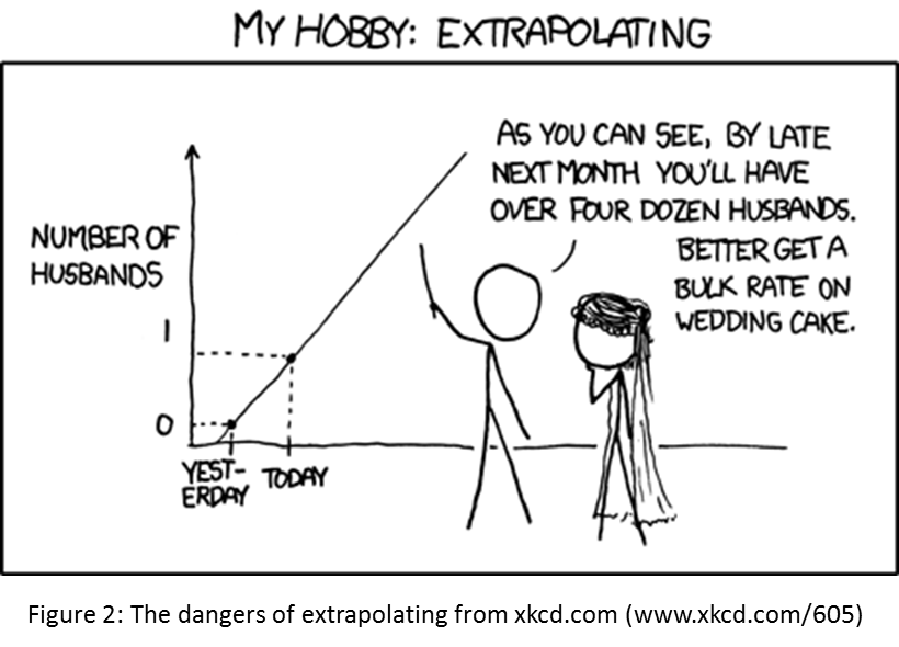
Most of the media attention that discusses ecosystem models focuses on predictions of ecosystem responses to climate change over the next century.  However, many of these models were built, parameterized, and tuned to work well for current conditions over a few decades, at most.  As scientists, we’ve all been warned about the dangers of extrapolating beyond the range for which we have data (Fig. 2).  With PalEON, we are working around this issue by simulating forest responses to past climate change from 850 A.D. through the present. Even though the empirical data for this time period is temporally and spatially sparse, it is better than the literal nothing available for models of the future.

One of the most eye-opening experiences for me has been the discovery that many ecosystem models actually can’t run for hundreds of years at a time.  Problems that prevent the models running can range from memory and computation limitations to the simulated thermodynamic physics in the model being impossible.  More on the challenges of long-term ecological modeling in the next installment: A day in the life of an ecological modeler.  (Spoiler alert: it involves lots of trial-and-error, communication, and XKCD cartoons.)


¹Here I specify simulation model to indicate a class of process-based models that can be given different scenarios (such as climatic conditions) that are used to predict a range of ecosystem states.  This contrasts with statistical models that are typically more descriptive in nature and lack explicit representation of processes such as photosynthesis or disturbance.


Edge of the Prairie

Posted by Jody Peters, PalEON Program Manager

Prior to major land use changes, the tall grass prairie was a widespread ecotone in North America extending east into Minnesota, Illinois and Indiana.  Caitlin Broderick, a

Figure 1. Study area. Townships within the Yellow River watershed.

University of Notre Dame undergraduate working in the McLachlan lab, wanted to learn more about the edge of the prairie this spring semester.  She could have listened to NPR’s Garrison Keillor describe life in Lake Wobegone on the edge of the prairie in Minnesota.  But given that Notre Dame has been compiling historical records of trees from Indiana and Illinois, she decided to look at bit closer to home and focused on townships that are within the Yellow River watershed.  Coincidentally, this watershed is split almost in two by what is currently US 31 and what was historically known in the Public Land Survey (PLS) notes as the Michigan Road Lands. (Fig 1).

The following are some of the results Caitlin presented at the University of Notre Dame College of Science Joint Annual Spring Meeting.

Prairie_Fig2Currently, the Yellow River region is dominated by agriculture and deciduous forests (Fig 2).  However, from a 1935 depiction of the extent of the prairie prior to Euro-American settlement, prairie ecosystems extended into northwest Indiana including into the Yellow River region (Fig 3; Transeau 1935).  Caitlin explored what the edge of the prairie in the Yellow River region looked like during 1829-1837 using historical forest data obtained from PLS.Prairie_Fig3The survey notes provide identification of 1-2 trees, their diameters and distances from corner posts set every mile in each township (n=30 townships; 1055 corners). For this study, trees at each corner were categorized as “Oak” (only oaks were present), “Other” (22 non-oak tree taxa which were dominated by beech, ash, maple and elms), or “Oak + Other” (a combination of oak and non-oak trees).  There were also corners that were categorized as “Water” (in lakes, rivers, creeks, etc.), “No Tree” (had a post set in a mound but with no trees nearby), or “No Data” (corners with no information provided in the notes).

Caitlin used Arc GIS to map the tree composition at each corner (Fig 4).  Much to our surprise, she did not see many corners with no trees in the areas of Transeau’s prairie in the Yellow River region.  However, there was a striking pattern in the distribution of the trees, with the majority of the trees to the west of the Michigan Road Lands being oaks and those to the east being other hardwoods.

Prairie_Fig4

In addition to examining tree composition, Caitlin wanted to look at the structure of the trees and the physical environment across the region. To better define the two groups of trees (Oaks to the west and Other hardwoods to the east), Caitlin created buffers around individual corners and dissolved the buffers with matching tree classifications to create two groups of trees (Fig 5A). Comparing the trees in the two groups, Caitlin found that there was no difference in tree diameter (mean (cm)± se; Oak: 40.9± 0.5; Other: 40.2± 0.6). However, the trees in the Oak group were significantly further from the corner posts compared to the Other group (mean (m)± se; Oak: 36.2± 4.3; Other: 13.6± 2.4; p<0.001).  Given that there was a difference in the tree composition and distance from the corners, Caitlin looked at climatic and physical features that could help explain this difference between the oaks of the west and the other hardwoods in the east.  There was no ecological difference in either temperature or precipitation (mean± se; Temperature (ºC): Oak: 9.88± 0.003; Other: 9.89± 0.003; Precipitation (mm): Oak: 1010± 0.59; Other: 1007± 0.74).  However, although northern Indiana is quite flat, as with the tree composition, there was a striking difference in the pattern of elevation change across the Yellow River region that mirrored the change in the tree distribution. Trees in the Oak group were at significantly lower elevation compared to trees in the Other group (mean (m)± se; Oak: 225.5± 0.7, Other: 251.0± 0.6; p<0.01; Fig 5B).

Prairie_Fig5ab

IPrairie_Fig6n addition to exploring what the historical prairie-forest boundary looked like, Caitlin compared the National Commodity Crop Productivity Index (NCCPI) to see if there is a lasting impact on the current crop production by the physical factors that contributed to the differences in historical tree composition and structure.  The NCCPI models the ability of soils, landscapes, and climates to foster non-irrigated commodity crop productivity (Dobos et al. 2012). Caitlin found there was in fact, a difference between NCCPI of the two groups with crop productivity being significantly lower in the western area historically dominated by low density Oak tree communities (Fig 6).

Typically when people think of prairies, they think of open expanses of grass.  However, over the spring semester Caitlin found that in the Yellow River region of northern Indiana, the prairie described by Transeau actually looked more like a low density oak community compared to the closed forests further east.  While at first glance we can no longer see the prairie’s edge in the current vegetation of northern Indiana (Fig 2), when Caitlin looked closer, the factors that once controlled the boundary between the closed forests of the east and the open savannas moving west may still be at work limiting crop production in what was once savanna compared to production in the historically wooded uplands (although what these factors specifically are is still an open question).

As a fun follow-up to Caitlin’s research, nine of us took a lab canoe trip down the Yellow River. Although we didn’t see the same striking pattern of oaks to the west and other hardwoods to the east, as we drove the 50 minutes south on US 31 to get to the River, we did see small stands of hardwoods intermingled with a number of lone oaks standing in the middle of corn and soybean fields.  On our way to the ice cream store after our canoe trip, we also saw some of the lasting impacts of the oak savannas as we drove through Burr Oak, Indiana.  According to McDonald (1908), the village plat was filed in 1882 and was “nearly in the center of what is known as the “Burr Oak Flats”, which is as beautiful and productive a region as can be found anywhere.”

The trip down the Yellow River was a wonderful way to get outside on a beautiful spring day and experience firsthand the watershed/ecosystem that Caitlin has spent this spring studying in the lab.  The river was an easy enough paddle that novice canoers would be comfortable, but had enough downed trees to provide excitement for the more experienced canoer.  If you are ever in the area, connect with the Little Bit Canoe Rental. They do a wonderful job providing canoes and transport. Here are a couple of pictures of the fun!

Prairie_Fig7


References

Dobos, R.R., H.R. Sinclair, Jr., M.P. Robotham. 2012. User Guide for the National Commodity Crop Productivity Index (NCCPI), Version 2.0. Access pdf at the bottom of the page here.

McDonald, D. 1908. A Twentieth Century History of Marshall County, Indiana, Volume 1. Lewis Publishing Company, pg 134. Online access here.

Transeau, E. N. 1935. The Prairie Peninsula. Ecology 16(3): 423-437.

Pollen Dispersal II: Quantitative Reconstructions

Post by Kevin Burke, Graduate Student at the University of Wisconsin, Madison working with Jack Williams.  

Since Lennart Von Post presented the first modern pollen diagram in 1916, the palynological community has been working to better understand the relationship between pollen abundances recovered from sediments, and the vegetation that produces this pollen.1,2 Throughout the twentieth century great strides have been made in quantitatively reconstructing past vegetation from relative pollen percentages. Mechanistic transport models by Colin Prentice and Shinya Sugita use taxonomic abundance and pollen productivity to estimate pollen source area, while other recent work by PalEON member Andria Dawson study this relationship using sophisticated Bayesian hierarchical models.3,4 However, these approaches all tend to use simplifying assumptions,  including constant, uniform wind speeds, and a circular source area. Our work here seeks to challenge and improve upon some of these underlying assumptions by developing a pollen transport model that includes realistic, variable wind speeds and directions.  Moreover, we are using the historical estimates of vegetation developed by the PalEON project.

Using North American Regional Reanalysis (NARR) wind data, a vegetation dataset of tree composition pre-Euro-American settlement , fossil pollen records from the Neotoma Paleoecology Database, and taxon-specific measurements of settling velocities for pollen grains, we are producing improved estimates of pollen loading (in grains per square meter) for lakes across the Prairie-Forest ecotone in the upper Midwest.  This work recently won an Outstanding Student Paper Award from the 2014 Fall Meeting of the American Geophysical Union.

Fig1

While the source area is largely governed by presence/absence of taxa in the vegetation dataset, things become much more interesting when looking at the ratio of relative proportion of pollen loading to relative proportion of trees per grid cell. We see that some taxa are much better represented in the pollen records given the number of trees on the landscape.

Fig2

We can also see that whether a given taxon is over- or underrepresented varies spatially, based on distance to lake and the other taxa present in a given grid cell.  These results shed light on the potential magnitude of a regional pollen source area, and help elucidate the relationship between pollen in a sediment core and trees on the landscape.  Ultimately, this kind of work can be used to build more accurate reconstructions of past vegetation from fossil pollen records.  From there, these paleovegetation reconstructions can be used to better constrain and improve terrestrial ecosystem models – a central goal of the PalEON project.

To see more results, including preliminary comparisons to pollen counts from sediment cores, you can check out our American Geophysical Union poster here.

References:

  1. Fries, M. Review of Palaeobotany and Palynology, 1967.
  2. Marquer et al. Quaternary Science Reviews, 2014.
  3. Prentice, C. Quaternary Research, 1985.
  4. Sugita, S. Quaternary Research, 1993.

2014 AGU PalEON Talks & Poster Schedule

If you are going to be at AGU next week, Dec 15-19. Be sure to see our PalEON-related presentations and posters. We can help fill up your schedule all week as we have people presenting everyday except Wednesday!

There are two PalEON related sessions being led by people in our group.

1. B24B Constraining Ecosystem Carbon Uptake and Long-Term Storage Using Models and Data II
Tuesday, December 16, 4:00 – 6:00 PM in Moscone West, 2002
Conveners: David Moore, Valerie Trouet, Ankur Desai, Michael Dietze

2. PP44B Understanding Uncertainties in Paleoclimate and Paleoecology: Age Models, Proxy Processes, and Beyond II
Thursday, December 18, 4:00 – 6:00 PM in Moscone West, 2010
Conveners: Connor Nolan, John Williams, Lorraine Lisiecki, Deborah Khider

The following is the schedule of PalEON presentations with the title, presenter, and session number. Presentations are color coded by location.

PalEON presentation & poster schedule for AGU 2014. Presentations are color coded by location.

PalEON presentation & poster schedule for AGU 2014. Presentations are color coded by location.

In case you are still looking for ways to fill up your time at AGU, we have a number of PalEON participants that will be discussing other work they are involved with. Drop by to see the range of projects PalEON-ites are up to.

Other, non-PalEON presentations & posters given by PalEON members. Presentations are color coded by location.

Other, non-PalEON presentations & posters given by PalEON members. Presentations are color coded by location.


In a New Light

Post by Neil Pederson, Senior Ecologist at Harvard Forest
Reposted from The BroadLeaf Papers

We all love the colors of autumn. Fall brings to mind the vivid reds, oranges, yellows, and deep purples of September and October. By November in the Northeast, the leaves are gone and the sky often tilts into various shades of pale grey. The weather can be bone-chilling in a damp kind of way. It can be a bad time to be in the field. November in New England was the closest I’ve ever been to hypothermia. I now relish fieldwork in November, however, because of its light. November Light has helped me see things in a new way.

Filtered Light. Photo: N. Pederson

Filtered Light. Photo: N. Pederson

The first time I experienced the long-lasting glow of November Light was late in my dissertation field campaign. I recently had some great luck with a collection from an old-growth forest and wanted to see if I could squeeze out a few more diamonds before I called it a dissertation (and work would be lit by fluorescent light).

Kevin was my most reliable volunteer field assistant. I could call at a moment’s notice to see if he wanted to hit the field. He always said yes.

We bolted to southeast Pennsylvania and the weather was on our side. Blue skies and warm temperatures. We scoured this tiny patch of old forest to see if I had missed much on a prior trip. Soon after a brief lunch, it became apparent that we had done about all that was possible in that forest and we were slipping into lazy. So, we leaned back, chatted, and stared at the vernal roof.

At some point I kept checking the time on my GPS. My eyes kept telling me it was getting late. In reality, it was just approaching mid-afternoon. It dawned on me that angle of the Earth in that part of the Northern Hemisphere was delivering us an ever-lasting gobstopper dose of diffuse light. It felt like “sunset” above the Arctic Circle during summer. The light was low and hitting at all kinds of slanted angles. Colors glowed. It was glorious.

At the same time, it dawned on us that we were south of the last glaciation. Elk, woolly mammoth, and other megafauna likely used the game trails we were using that day more than a 100,000 years ago. More glory.

Bronzed Canopy. Photo: N. Pederson

Bronzed Canopy. Photo: N. Pederson

Just this past week we rolled up our field tapes for the last time during the 2014 PalEON season. It was a glorious feeling. Putting in ecological plots for tree-ring analysis is long and rather repetitive work. It is exhausting in a deeply different way than to reconstruct climate from tree rings. It was nice to know we had done a ton of work this year and that we were done. I imagine farmers get these feelings this time of year, too. As I dropped a coiled field tape into a backpack, it was instantly satisfying. We were putting our loyal field equipment down for a long winter’s rest.

Dan Bishop and Javier Martin Fernandez sampling in November Light. Photo: N. Pederson

Dan Bishop and Javier Martin Fernandez sampling in November Light. Photo: N. Pederson

We scheduled this last field campaign more than a month in advance. It is risky scheduling that far in advance in central New England this late in the year. But, after a Nor’Easter and a cold snap, the atmosphere shifted in our favor.

Blue skies. Brilliant Fagaceae colors. Stark contrast of a wide range of brightly-lit yellow leaves with the dark bark of red oak… and black oak?

While installing ‘nests’ around an older plot, or as a rather poetic colleague termed it, installing ‘doughnuts’, I ‘discovered’ a new species. Of course, black oak (Quercus velutina) was always there. It was just not talked about as much and, being hard to identify and often hybridizing with northern red oak Quercus rubra), it is often put in the red oak category. But, there it was, right in front our eyes.

Black oak reaching for the upper canopy among towering northern red oaks. Photo: N. Pederson

Black oak reaching for the upper canopy among towering northern red oaks. Photo: N. Pederson

Black oak bark. Photo: N. Pederson

Black oak bark. Photo: N. Pederson

Perhaps it was the November Light that made it ‘appear’? Maybe it was the showering of diffuse, angled light that made black oak jump out of the forest. Whatever it was, I now saw black oak everywhere. It wasn’t, of course. It was often red oak borrowing some of the velutinous traits of its sleeker, rarer cousin.

The glorious nature of November returned this past week and I saw these forests in a new light.

Canopy dominant red oak. Photo: N. Pederson

Canopy dominant red oak. Photo: N. Pederson

Classic red oak bark, bronzed. Photo: N. Pederson

Classic red oak bark, bronzed. Photo: N. Pederson

Oh there are some conifers in this forest (Pinus strobus). Photo: N. Pederson

Oh there are some conifers in this forest (Pinus strobus). Photo: N. Pederson

Glowing American beech (Fagus grandifolia). Photo: N. Pederson

Glowing American beech (Fagus grandifolia). Photo: N. Pederson

American beech. Photo: N. Pederson

American beech. Photo: N. Pederson

It comes in bronze, too. Photo: N. Pederson

It comes in bronze, too. Photo: N. Pederson

Fading Light. Photo: N. Pederson

Fading Light. Photo: N. Pederson

Late November Light. Photo: N. Pederson

Late November Light. Photo: N. Pederson

Pollen Dispersal I: Why We Get Sediment Pollen

Post by Andria Dawson, Post-Doc at University of California-Berkeley

Pollen and seed dispersal are important reproductive processes in plants, and in part determines the abundance and extent of a species. With a recent push to understand how species will respond to global climate change, dispersal ecology has gained increasing interest. We really want to know if there is a dispersal limitation, or if species can migrate quickly enough to maintain survival in a changing environment. Addressing this question presents challenges, many of which arise from trying to understand and quantify dispersal in ecosystems that are changing in both space and time (Robledo-Arnuncio 2014).
Pollen
In PalEON, one of our efforts involves estimating the past relative abundance of vegetation from fossil pollen records. To do this, we need to quantify the pollen-vegetation relationship, which includes modelling pollen dispersal processes.

For many trees, including those we study in the PalEON domain, pollination is exclusively (or at least predominantly) anemophilous (carried out by wind). In angiosperms, wind pollination is thought to have evolved as an alternative means of reproduction for use when animal pollinators are scarce (Cox 1991). It was previously understood that wind pollination was less efficient than insect pollination (Ackerman 2000), but Friedman and Barrett (2009) show that may not be the case. To estimate the efficiency of wind pollination, they compared pollen captured by stigmas to pollen produced, and found that the mean pollen capture was about 0.32%, which is similar to estimates of animal pollination efficiency. Although both dispersal vectors are comparable with respect to efficiency, these quantities indicate that both are still pretty inefficient – this is great news for paleoecologists! Some of the pollen that is not captured ends up in the sediment.

Now we know that we expect to find pollen in the sediment, but how do we begin to quantify how much pollen of any type we expect to find at a given location? The route a pollen grain takes to arrive at its final location is governed by atmopsheric flow dynamics (among other things). These dynamics are complicated by landscape heterogeneity and climate, and differ among and within individuals because not all pollen grains are created equal. However, we usually aren’t as interested in the route as we are in the final location – in particular, we want to know the dispersal location relative to the source location. The distributions of dispersal locations from a source defines a dispersal kernel which can be empirically estimated with dispersal location data. Often these kernels are modelled using parametric distributions, usually isotropic, and often stationary with respect both space and time. Are these approximations adequate? If so, at what scale? These are some of the questions we hope to address by using Bayesian hierarchical modelling to quantify the pollen vegetation relationship in the Upper Midwest.

References
1. Robledo-Arnuncio, JJ, et al. Movement Ecology, 2014.
2. Cox, PA. Philosophical Transactions of the Royal Society B: Biological Sciences, 1991.
3. Friedman, J, Barrett SCH. Annals of Botany, 2009.
4. Ackerman, JD. Plant Systematics and Evolution, 2000.

Underwater In New England

Post by Bryan Shuman, Associate Professor of Geology & Geophysics at the University of Wyoming

To evaluate how forests have responded to climate change in the past, we need to reconstruct the climate history. Fortunately, in terms of moisture, lakes provide a geological gauge of precipitation (P) minus evapotranspiration (ET). As effective moisture (P-ET) changes, the water tables and lake surfaces rise and fall in elevation. When this happens, sands and other materials that typically accumulate near the shore of a lake are either moved deeper into the lake during low water or shift out from the lake’s center as water levels rise. Ongoing work in New England is building on existing datasets to provide a detailed picture of the multi-century trends in effective moisture. Here are a few highlights of recent progress.

First “the fun part” was fieldwork that I conducted while on sabbatical in New England. The work included a cold but fun day on the ice of Twin Pond in central Vermont with Laurie Grigg and students from Norwich University (pictured).

Coring at Twin Ponds

Coring at Twin Ponds

This trip was a follow up to a previous trip that coincided with Hurricane Sandy’s visit to New England in 2012. As the result of both trips, we now have a series of three cores that record shoreline fluctuations at the pond. Because the sediment contains both carbonate minerals and organic compounds, we have also been able to examine the ratios of oxygen and hydrogen isotopes in the sediment and provide some constraints on the temperature history too.

Ice makes coring easy (its stable), but the swimming was not as good as in the summer when I worked in southern New England with Wyatt Oswald (Emerson College), Elaine Doughty (Harvard Forest), and one of Harvard Forest’s REU students, Maria Orbay-Cerrato. Over several days, we collected new cores that record the Holocene water-level changes at West Side Pond in Goshen, Connecticut, and Green Pond, near Montague, Massachusetts. Floating on a pair of canoes, we enjoyed the early summer sun, told jokes, ate delightful snacks brought from home by Wyatt, and strained our muscles to pull about 5 cores out of each lake. Near shore, the cores from both lakes contained alternating layers of sand and mud consistent with fluctuating water levels. In the lake center at West Side Pond, we also obtained two overlapping cores about 14 m long, which promise to provide a detailed pollen record. Both lakes proved to be excellent swimming holes too!

Second, on a more earnest note, the existing geological records of lake-level change from Massachusetts have been synthesized in a recent (2014) paper in Geophysical Research Letters by Paige Newby et al. The figure shown here summarizes the results and compares the reconstructions with the pollen-inferred deviation from modern annual precipitation levels from a paper by University of Wyoming graduate student, Jeremiah Marsicek, last year (2013) in Quaternary Science Reviews.

Figure 4 from Newby et al. 2014

Figure 4 from Newby et al. 2014

All of the records show a long-term rise in effective moisture since >7000 years ago as well as meaningful multi-century deviations. By accounting for the age uncertainties from the reconstructions, we were able to show that a series of 100-800 year long droughts at 4200-3900, 2900-2100, and 1300-1200 years before AD 1950 affected lake levels (blue curves with reconstruction uncertainty shown) on Cape Cod (Deep Pond), the coastal Plymouth area (New Long Pond), and the inland Berkshire Hills (Davis Pond) – as well as the forest composition as recorded by the pollen from Deep Pond (red line). Interestingly, an earlier drought in the Berkshires at 5700-4900 years ago was out of phase with high water recorded in the eastern lakes. This difference is one of the motivations for the new work in Vermont, Connecticut and central Massachusetts, as well as other ongoing work with Connor Nolan in central Maine: what are the spatial patterns of drought?

The Magic of Science is its Complexity

Post by Lizzy Hare, sociocultural PhD student at the University of California, Santa Cruz. Her dissertation research is on the contributions of paleosciences to the development of forecast models that could be used for policy and management. PalEON is one component of her dissertation.

As an anthropologist of science, my goal is to try to discourage obsolete and idealized views of science through the development of more open and realistic accounts. My training is in cultural anthropology, a sub-discipline that has traditionally worked through the medium of ethnography – descriptive accounts of the customs and practices of people and cultures.

Credit: Climate Change Encyclopedia

Credit: Climate Change Encyclopedia

In my research, I am learning about the process of producing scientific knowledge about climate change adaptation so that I may write about this for a general audience. I hope to share the daily practices, the complexities, the passions, the concerns, as well as the monotony, the frustration and the many absolutely mundane decisions that go on “behind the scenes” of knowledge production, so that we can move beyond idealized understandings of science that have caused political trouble around issues pertaining to climate change adaptation.

There is a great body of information that could aid policymakers and land managers in developing climate change adaptation strategies, but the political climate is such that the issue is avoided, as if ignoring it will make it go away, or is discussed obliquely, as in Florida governor Rick Scott’s recent efforts to begin to address the consequences of climate change without mentioning its causes.

Credit: Rice University/Photos.com

Credit: Rice University/Photos.com

Part of the problem is declining trust in science by those who identify as politically conservative or moderate (Gauchat 2012). But thinking of the issue as simply a matter of conservatives versus liberals is a gross oversimplification. This is a part of the same cultural phenomenon that has led educated, high-income (and generally politically liberal) mothers to opt out of childhood vaccination schedules (Reich 2014). Both climate change skeptics and anti-vaxxers eschew scientific consensus, favoring instead the right to individual freedom to weigh evidence and make independent decisions. Adherents of this position see their method of knowledge acquisition (through shared first-hand accounts, anecdotal evidence, and sometimes even religious texts) to be equivalent to that produced in mainstream science.
Further, because it has become such a politically contentious topic, the polemics on both sides can make it difficult to take seriously those with dissenting opinions. Politicians with largely anti-science constituencies, such as Senator Coburn, have found it politically advantageous to scrutinize science in general and the NSF in particular, and the findings of his report were mocked in the conservative-serving media. On the other side of the spectrum, Michael Mann’s pugnacious and often condescending public persona demonstrates an utter disinterest in the reasons why people choose not to follow science.

Anthropologist of science, Myanna Lahsen and self-described conservative journalist Pascal-Emmanuel Gobry have written about how the public’s idealized perception of science contributes to the contention. According to Lahsen (2013) and Gobry, the public generally believes that science should be an objective broker of truth, independent of culture and politics. Members of the public are thus understandably confused, frustrated, and skeptical when scientific findings emphasize uncertainty or change from year to year or get involved in heated political debates. After all, if they are brokering in absolute Truth, a scientific finding would be the final word on a matter. Lahsen, following anthropologist Christopher Tourney (1996) calls the belief in an idealized science “scientific fundamentalism”. Gobry simply and more bluntly calls it a “botched” understanding of science.

Whether you see the idealized understanding of science as fundamentalist or flawed is relatively inconsequential. Of more immediate concern are the unrealistic expectations that these idealized understandings place on scientific findings. Not only do they discount the tremendous amount of work that goes into continually adjusting, refining, and occasionally revolutionizing scientific knowledge, but they also set up an expectation that science should be wholly without cultural or political influence. This is something that science simply cannot do. Lahsen (2013) shows how unrealistic expectations of science made the Climategate controversy more problematic than it ought to have been, because the “troubling” material that the hackers found in the Climatic Research Unit’s emails can only be considered problematic if there is an a priori assumption that science does not include making subjective decisions about data, analysis, and findings. Following Climategate, contrarian interpretations of climate change gained support in the United States, because it produced evidence that mainstream science is “flawed” by politics and therefore cannot produce Truth (capital T). If this is the case, so the logic goes, then other politically-motivated interpretations of science must be equally valid. (A great example of this kind of interpretative symmetry can be found in the Heartland Institute’s response to the article by Jank³ et al. (2014) that PalEON member Simon Goring described in his blog posts here).

To try to put an end to this argument, the belief that science is a perfect, objective, apolitical, knowledge-producing machine needs to be laid to rest. In place of that narrative we need one that explains the awesome, dynamic complexity of science in practice. There is absolutely no reason for why we need to exaggerate or make science appear magical, the history of science is truly impressive. After all, science has made possible unprecedented advances in knowledge, technology and quality of life.

References Cited:

Gauchat, G. (2012). Politicization of Science in the Public Sphere: A Study of Public Trust in the United States, 1974-2010. American Sociological Review 77(2):167-187.
Lahsen, M. (2013). Climategate: The role of the Social Sciences. Climatic Change 119:547-558.
Reich, J. (2014). Neoliberal Mothering and Vaccine Refusal: Imagined Gated Communities and the Privilege of Choice. Gender & Society 28(5):679-704.
Tourney, C. (1996). Conjuring Science: Scientific Symbols and Cultural Meanings in American Life. Rutgers University Press: New Brunswick.

Big process, small data: Reconstructing climate from historical U.S. fort data

Post by John Tipton, statistics graduate student with Mevin Hooten at Colorado State University, about work John and Mevin are doing with Jack Williams and Simon Goring.

Big data” has very rapidly become a popular topic. What are big data? The concept of big data in statistics is the analysis of very large datasets with the goal of obtaining inference in a reasonable time frame. The paleoclimate world often has the opposite problem: taking small amounts of data and expanding to produce a spatially and temporally rich result while accounting for uncertainty. How do you take a handful of temperature observations and predict a temperature surface over 20,000 locations for a period of 73 years in the past? Perhaps some of the techniques used in big data analysis can help.

Figure 1. Four representative years of temperature records (ºC) from the historical fort network.

Figure 1. Four representative years of temperature records (ºC) from the historical fort network.

The U.S. fort data consist of temperature records from military forts in the Upper Midwest region of the United States from 1820-1893. A subset of these instrumental temperature records (Figure 1) illustrates the sparse nature of the historical U.S. fort data relative to the spatial area of interest, especially in the earlier two years (1831 and 1847). From the small set of temperature observations collected each year, we seek to reconstruct average July temperature at a fine grid of 20,000 prediction locations. Techniques such as optimal spatial prediction, dimension reduction, and regularization allow us to provide formal statistical inference for this very large underlying process using a relatively small set of observational data.

To ameliorate the sparsity of the fort data, we used patterns from recent temperature fields (i.e., PRISM products) as a predictor variables in a Bayesian hierarchical empirical orthogonal function regression that includes a correlated spatial random effect. A strength of this modeling technique is that the primary patterns of temperature should remain stable even though the magnitude might change (e.g., it will always be cooler in the north than in the south). Another characteristic of this methodology is that it allows for localized differences in prediction to arise through a correlated spatial random effect. The correlated spatial random effect is too computationally expensive to calculate using traditional methods so the effect is estimated using big data techniques. Specifically, any remaining correlation that ties the fort locations together beyond that predicted by combinations of the primary temperature patterns is approximated in a lower dimensional space. This greatly reduces the computational effort needed to fit the model. We also employ a type of model selection technique called regularization to borrow strength from years with more data. This results in predictions that are close to the historical mean when there are few observations in a given year, while allowing for more detailed predictions in years with more data. To make the model selection computationally feasible, we fit the model in a highly parallelized high performance cluster computing environment.

The use of big data techniques for large paleoclimate reconstruction allows for statistical estimation of climate surfaces with spatially explicit uncertainties. Results of the mean July temperature for the subset of four years are shown in Figure 2, while the associated spatially explicit uncertainties are shown in Figure 3. These figures illustrate the strengths of the modeling techniques used. In the two earlier years, the predictions are similar to the historical mean with uncertainty increasing as a function of distance from observations. In the two later years with more data, the predictive surfaces have more spatial complexity and less associated uncertainty.

Figure 2. Reconstruction based on the posterior mean July temperature (ºC) for four representative years of the historical fort network.

Figure 2. Reconstruction based on the posterior mean July temperature (ºC) for four representative years of the historical fort network.

Figure 3. Posterior standard deviation surface of mean July temperature (ºC) for four representative years of the historical fort network.

Figure 3. Posterior standard deviation surface of mean July temperature (ºC) for four representative years of the historical fort network.

By explicitly accounting for latent correlated spatial structure and moderating model complexity using regularization, spatio-temporal predictions of paleoclimate are improved. Furthermore, dig data techniques allow us to fit the statistical models in a reasonable time frame (i.e., on the order of days rather than weeks). The relatively small sample sizes commonly associated with paleoclimate data would not normally fall into the “big data” realm of analyses. However, the processes on which we seek inference are quite large, and thus “big data” techniques are tremendously helpful.


Quaternary Science . . . on Mars . . . three billion years ago.

Post by Simon Goring, Research Assistant at the University of Wisconsin, Madison
Originally posted on OpenQuaternary Discussions.

For a curious person, one of the great benefits of being a Quaternary researcher is the breadth of research that is relevant to your own research questions.  The recent publication of fifty key questions in paleoecology (Seddon et al., 2014) reflects this breadth, spanning a broad range questions that reflect human needs, biogeophysical processes, ecological processes and a broad range of other issues.  The editorial board of Open Quaternary also reflects this incredible disciplinary breadth.  To me it is clear that the Quaternary sciences is an amalgam of multiple disciplines, and, at the same time, a broadly interdisciplinary pursuit.  To be successful one must maintain deep disciplinary knowledge in a core topic, as well as disciplinary breadth across topics such as ecology, anthropology, geology (and specifically geochronology), and you need a good grounding in statistics and climatology.

One of the things that is not always quite as apparent is the breadth of research affected by the Quaternary sciences.  My first exposure to the utility of paleoecology for understanding interplanetary dynamics came as the result of a paper we published two years ago.  In 2012, my co-authors and I developed a regional scale estimate of sediment deposition times in lakes across eastern North America for the Holocene (Goring et al, 2012). We did this because we were looking toward re-building age models for all cores in eastern North America and wanted to use reliable priors for Bacon (Blaauw and Christen, 2011).  Our priors wound up becoming the default in Bacon, which is great, but the results have also helped inform the lacustrine history of the red planet, Mars.


Figure 1. Paleo-lake level reconstruction in the Melas Baisn of Mars. From Williams and Weitz (2014).

Williams and Weitz (2014) were examining the Melas Basin, a feature of the Martian surface that appears to show evidence of lacustrine activity at some time in the past. Given a set of lacustrine features and channel beds in the basin, they began the process of trying to reconstruct lacustrine activity on the surface of Mars. It seems clear that if our own understanding of geophysical processes during the Quaternary is based on Whewell and Lyell’s concept of Uniformitarianism, that uniformity of process should not be limited to earth.

While we might assume uniformity, there are limits to how much modern or paleo terrestrial analysis can be applied to the Martian surface. Although the basin age is dated roughly using meteor strikes, the dating of lacustrine establishment and termination are much more difficult. For one, Holocene models rely on 14C dates. While it may be possible to obtain some form of geochronological information from the Martian surface, at some point it likely requires dating techniques we don’t have on hand.  However, researchers can develop experimental procedures to test the possibility of using other dating techniques, and it seems like development of these techniques is already underway with K-Ar dating (Hurowitz et al., 2012, PDF).

Another limitation of using Quaternary analysis is that our Holocene estimates rely on the assumption that there is near-modern vegetation cover, that sediment transport and flow rates are similar to modern and the distribution and types of sediment are similar to modern. Even in this assumption we know there are exceptions. Sediments deposited immediately following deglaciation are often very fine grained, we often see strong increases in organic content during the Holocene, and the presence of a major inflection point in deposition rates is a persistent feature of the near-modern era.

Regardless, to understand how long a lake was present in the Melas Basin there are few options but to look at earth systems. The Williams and Weitz paper (2014) looked at both deltaic sediments and lake sediments in the basin. Williams and Weitz (2014) estimate lacustrine activity using sedimentation rates from large deltas in the United States and Russia and our sedimentation rates for lacustrine environments. Interestingly, the deltaic sedimentation and lacustrine sedimentation rates seem off by orders of magnitude. In Goring et al. (2012) we show a mean sedimentation rate of approximately 20yr/cm, meaning the lacustrine environments of the Melas Basin might have persisted for almost 90,000 years, while sedimentation rates from the deltas produce estimates of between 1,000 and 4,000 years.

In a Holocene or Quaternary context, orders of magnitude between 1,000 and 100,000 seem incredibly broad. But, when we consider that we are examining the surface of another planet, and that the lake formation dates to the Hesperian period almost 3 billion years ago, the temporal certainty that Quaternary science can provide for interplanetary research is in fact astounding.

References Cited:

Blaauw, M, & Christen, JA (2011). Flexible paleoclimate age-depth models using an autoregressive gamma process. Bayesian Analysis6(3), 457-474.

Hurowitz, JA, et al. (2012). A New Approach to In-Situ K-Ar Geochronology. LPI Contributions, 1683, 1146.

Goring, S, et al. (2012). Deposition times in the northeastern United States during the Holocene: establishing valid priors for Bayesian age models.Quaternary Science Reviews,48, 54-60.

Seddon, AW, et al. (2014). Looking forward through the past: identification of 50 priority research questions in palaeoecology. Journal of Ecology102(1), 256-267.