Synthesizing Fire-History Records to Understand Fire-Regime Variability Across Alaska

Post by Tyler Hoecker graduate student with Philip Higuera at the University of Montana. Tyler received an Outstanding Student Paper Award when he presented this work at AGU 2015!

Over the past two decades the paleoecological research community has amassed dozens of sediment cores from across Alaska. These long-term records contain a range of clues about the character of ecosystems and climate that existed deep in the past. Some records extend back as far as 14,000 years, and have been used to reconstruct millennial-scale vegetation, climate and disturbance dynamics. For example, Higuera et al. (2009) identified the marked increase in biomass burning and fire frequency following the transition from forest-tundra to modern black-spruce dominated boreal forest ca. 5000-6000 years ago using cores from four lakes in the south-central Brooks Range (Figure 1).

Figure 1

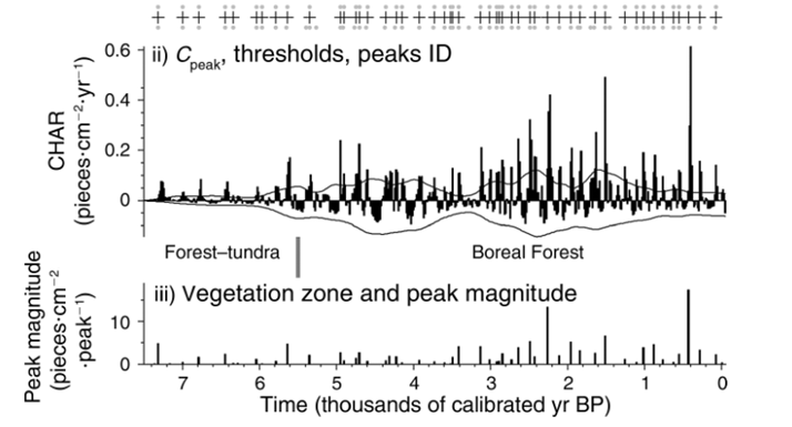
Figure 1. Paleocharcoal record from a south-central Brooks Range lake presented in Higuera et al. 2009. Vertical bars in the top panel show the charcoal accumulation rate (CHAR; pieces cm-2 year-1) over the past 7,000 years, and crosses indicate peaks in CHAR that are inferred to represent local fire events. Bottom panel shows peak magnitude (pieces cm-2 peak-1) delineated by vegetation zone.

More recent work has focused in on the past two millennia to understand the sensitivity of fire regimes in the boreal forest to centennial-scale climate change, including the Medieval Climate Anomaly (MCA) and the Little Ice Age (LIA) (Kelly et al., 2013). Persisting from ca. 850-1200 A.D. (750-1100 calibrated years before present), the MCA has been proposed as a rough analog to modern and predicted climate warming. This work identified significant increases in biomass burning during the MCA based on 14 cores from the Yukon Flats region of boreal forest, likely in response to regional warming. Biomass burning tapered off before LIA cooling began, hypothesized to reflect negative feedbacks from fuel limitations (Kelly et al., 2013).

The synthesis work I presented at AGU built on the work of Kelly et al. (2013) and focused on characterizing centennial-scale variability over the past two millennia in an additional 12 published fire-history records from elsewhere in the Alaskan boreal forest and tundra (Copper River Basin, Brooks Range, Noatak River Watershed). I looked at these records as Alaskan-wide (n=26) and regional composites (n=14 in Yukon Flats and n=4 elsewhere).

Figure 2

Figure 2. Maps of new and published paleocharcoal records used in the synthesis. 26 paleocharcoal records were analyzed as an Alaskan-wide composite, and as ecoregional composites (colored polygons). 8 new records were collected in the Kuskokwim Mountains ecoregion of interior boreal forest (dark green polygon, westernmost points) in June 2015. Wildfire burn perimeters since 1939 are shown in red.

Each of the composite records demonstrates the pronounced high-frequency variability in fire activity, but long-term trends were also revealed. As an Alaskan-wide composite, this analysis suggests a relatively cohesive increase in biomass burning during the MCA, and a reduction during the LIA, largely reflecting the influence of the Yukon Flats records (Figure 3).

Figure 3

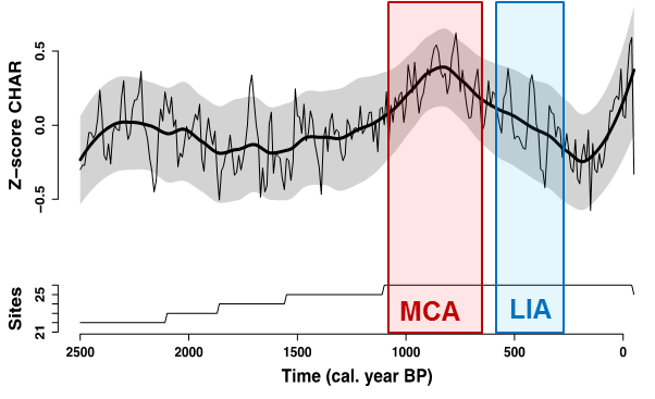
Figure 3. Alaskan-wide composite of 26 paleocharcoal records. Top panel shows the Z-score of charcoal accumulation rate (CHAR; pieces cm-2 year-1) over the last 2500 years. Thick black line represents a 500-year mean, thin black line represents a 100-year mean, and gray band indicates bootstrapped 90% confidence intervals around the 500-year mean. Colored bars indicate the approximate persistence of the Medieval Climate Anomaly (MCA) and Little Ice Age (LIA). Bottom panel indicates the number of records contributing to the composite through time (22-26).

When considered as regional composites (Figure 4) variability across Alaska emerges. At this scale the Yukons Flats, Copper River Basin, and Noatak River Watershed all show a sensitivity to warming, with some variability in the timing of this response. However, the Brooks Range sites show little low-frequency variability during either the MCA or LIA. This suggests that vegetation feedbacks or regional-scale controls act to moderate the impact of warming on biomass burning. Alternatively, climate forcing could have been uneven across Alaska as this scale, and/or climate forcing may not have been substantial enough in some regions to elicit a response in fire regimes. The sensitivity in observed paleocharcoal records may also be a function of sample size; centennial-scale change in some regions may be subtler than can be detected with only four lake cores.

Figure 4

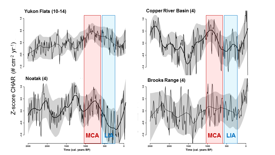
Figure 4. Regional composite paleocharcoal records. Time series are labeled by region (number of records). Each shows the Z-score of charcoal accumulation rate (CHAR; pieces cm-2 year-1) over the last 2500 years. Thick black line represents a 500-year mean, thin black line represents a 100-year mean, and gray band indicates bootstrapped 90% confidence intervals around the 500-year mean. Colored bars indicate the approximate persistence of the Medieval Climate Anomaly (MCA) and Little Ice Age (LIA).

Untangling the potential mechanisms driving the variability across time and space will require similar analyses with larger datasets. For my PalEON-supported MS thesis I will incorporate eight new lake-sediment records collected in 2015 to assess fire-regime sensitivity in a climatically distinct region (Figure 2). This network of lakes will lend itself to detecting the relatively short-term variability of the MCA and LIA. Spatially explicit reconstructions of climate over this time period will also help to explain the causes of variability in biomass burning, and improve our understanding of the relative importance of climate and vegetation dynamics in driving fire regime trend.

Citations
Higuera et al. 2009. Vegetation mediated the impacts of postglacial climate change on fire regimes in the south-central Brooks Range, Alaska. Ecological Monographs 79(2): 201-219

Kelly et al. 2013. Recent burning of boreal forests exceeds fire regime limits of the past 10,000 years. Proceedings of the National Academy of Sciences 110(32): 13055-13060

Science at Notre Dame

Post by Jody Peters, PalEON Program Manager

While PalEON members come from a multitude of institutions from around the US and across the globe, there are a number of individuals based at the University of Notre Dame. Here at Notre Dame we are remembering Father Ted’s impact on the growth and development of scientific research at ND.

To learn about Father Hesburgh’s influence see: http://research.nd.edu/news/64738-hesburghs-influence-on-science-at-notre-dame/

Empirically Reconstructing Biophysics with Remote Sensing Data

Post by Bethany Blakely graduate student with Adrian Rocha and Jason McLachlan at the University of Notre Dame

Biophysics is important . . . but only recently!

The exchange of energy between the land surface and the atmosphere (biophysics) plays a huge role in local and global climate. The polar ice-albedo feedback, where snowmelt reduces albedo and further accelerates melting, is an example that most readers will be familiar with. Vegetation is an important mediator of biophysical change (Figure 1). Changes in stature, phenology, water use, and other vegetation characteristics alter the exchange of energy between a vegetated surface and the surrounding atmosphere. Despite the potential climatic importance of these effects, they were often neglected in early efforts to understand vegetation-climate interactions. One contributor to the relative neglect of biophysics in past climate science may be its temporospatial misalignment with vegetation processes. Surface-atmosphere energy exchanges happen rapidly and at a local scale, making them hard to rectify with annual to centennial changes in landscape and climate.

Figure 1

Figure 1. Major ways in which vegetation affects surface-atmosphere exchange of energy. CRO = crops, DBF = deciduous broadleaf forests, ENF = evergreen needleleaf forests, GRA = grassland. Forested land tends to absorb more energy than non-forested land due to lower albedo but dissipates a larger portion of that energy through evaporation, limiting temperature increase. Zhao et al 2014


Remote sensing to the rescue?

Remote sensing is a useful tool for bridging the gap between biophysical and landscape processes. It offers a great deal flexibility in scale and is well suited to represent the kinds of things that matter for biophysics. After all, remote sensing satellites literally measure outputs of energy from the land surface. Since the processed data products from these measurements are standardized at relatively fine temporospatial resolution but collected over annual to decadal periods of time, they facilitate highly data-informed generalizations about fine-scale processes.

The biophysics of the past

I’ve been spending the past two years using “okay, mostly learning to use” remote sensing data to empirically link vegetation and biophysics. The goal is to understand how vegetation change since European settlement has altered the biophysics of the land surface, and how that might affect climate.

Fig 2

Figure 2: PLS pre-settlement vegetation and MODIS modern vegetation

I used 10-year averages of MODIS remote sensing data to create regressions linking vegetation type to two important biophysical properties: albedo and surface temperature. I then projected that relationship onto the vegetation of the past. Think 30,000-color paint-by-number grid cells.

Fig 3

Figure 3: Differences (modern vs historic) in albedo and surface temperature

The biophysical changes in the land surface are striking. Typical albedo has increased in the winter – there are less trees (because of logging, urban expansion, etc.) to cover up the snow – but is mostly unchanged in the growing season. Surface temperature has decreased in winter but increased in summer. This trend is particularly interesting because it seems to suggest a loss of temperature regulation with the loss of forests; the modern surface is colder in the cold season and warmer in the warm season. For more detail on my findings, check out my recent AGU poster. Although we can’t know exactly how a centuries-gone landscape exchanged energy with its atmosphere, remote sensing data offers a way to construct useful empirical baseline for changes in vegetation biophysics. In addition to offering its own scientific insights, this work could serve as an interesting comparison to outputs from Paleon Models, a role which I plan to participate in on in the upcoming site level model intercomparison project.

Reconstructing Multivariate Climate Using A Mechanistic Tree Ring Model

Post by John Tipton, statistics graduate student with Mevin Hooten at Colorado State University

Statistical Challenges of Paleoclimate Reconstructions
The ability to reconstruct paleoclimate from proxy data is important for understanding how climate has changed in the past and to allow exploration into how changing climate influences ecological processes. Statistical reconstructions of paleoclimate have unique challenges because proxy data are noisy, indirect observations of climate. Thus, any statistical model must address the following challenges: change of temporal support, sparse data, and the prediction of unobserved climate variables. When reconstructing climate from tree ring widths, the change of temporal support arises because our climate data are monthly average temperature and log total precipitation, whereas tree ring growth is measured on an annual scale. Therefore, any statistical model must account for this temporal misalignment. To overcome estimation issues common in sparse data scenarios, many previous reconstructions used linear statistical methods with constraints to regress the tree ring widths onto climate. For a multivariate climate reconstruction (e.g., temperature and precipitation), predicting paleoclimate using linear regression requires the inversion of a many to one functional that has potentially infinite solutions. Thus, multivariate climate reconstructions from univariate tree ring width time series are not commonly performed.

Mechanistic Models – A Promising Alternative
There is a need for rigorous statistical multivariate climate reconstructions, and hence, we developed an alternative to using linear statistical methods (Tipton et. al., In Press), using a mechanistic, biologically motivated model that “grows” tree rings to approximate the true growth process. By growing tree ring widths on a monthly time step, the mechanistic model aligns the monthly climate data with annual tree ring width data. Extending the mechanistic model to allow each tree species to have differential response to climate provides strong constraints on possible climate scenarios, ameliorating the difficulties that arise from having too many unknowns. We perform Bayesian inference to generate a probabilistic reconstruction that allows visual exploration of uncertainties. In contrast, many paleoclimate reconstructions generate point estimates that are not probabilistic in nature. The probabilistic reconstructions provide auxillary information that can be used to determine at what time periods the reconstruction is informative. Unfortunately, the use of a mechanistic growth model comes at a computational cost, thus we fit our model using Markov Chain Monte Carlo with compiled C++ code to increase computation speed.

Reconstruction of T and P – at the Same Time!
Our motivating goal was to generate a reconstruction of spatially explicit climate (temperature and precipitation) in the Northeastern United States that can be used to better understand how vegetation patterns have changed due to both climate change and direct human activity. Our work focuses on the Hudson Valley of New York, although in future work this model framework could be extended to the entire Northeastern United States. We focus on the Hudson Valley because there has been previous efforts to reconstruct the Palmer Drought Severity Index (PDSI), a combination of temperature and precipitation, which we can directly compare to our reconstruction, exploring the benefits and costs of different modeling frameworks. Figure 1 shows our joint temperature and precipitation reconstruction with the darkness of the shaded areas proportional to the probabilistic model predictions. For comparison, the black line in the log precipitation plot represents the previous centered and scaled PDSI reconstruction. Interestingly, there is little learning about temperature from our model (although the uncertainties are reasonable) while the log precipitation reconstruction is highly correlated (r=0.72) with the preexisting PDSI reconstruction. This result is in line with ecological expectations – drought in the Hudson Valley is strongly associated with precipitation (Pederson et al., 2015). When comparing our reconstruction to the previous efforts, our method has the added benefit of providing uncertainty estimates that illuminate where in time the reconstruction is informative without relying on statistically improper scoring rules like RE and CE commonly used in the paleoclimate literature. The use of proper scoring rules for assessing predictive ability is vital, because improper scoring rules can lead to incorrect inference about predictive skill.

Figure 1. Plot of probabilistic reconstruction of temperature and log precipitation using a mechanistic tree ring growth model. The reconstructions are shaded according to posterior predictive probabilities with the dotted lines giving the 95% credible interval. The solid black line in the log precipitation plot is a centered and scaled reconstruction of PDSI using the same data. The black lines at the far right of each reconstruction are the observational records.

Figure 1. Plot of probabilistic reconstruction of temperature and log precipitation using a mechanistic tree ring growth model. The reconstructions are shaded according to posterior predictive probabilities with the dotted lines giving the 95% credible interval. The solid black line in the log precipitation plot is a centered and scaled reconstruction of PDSI using the same data. The black lines at the far right of each reconstruction are the observational records.

What Did We Learn?
Reconstructing climate based on ecological proxies is tricky! Our simulations showed that the model we developed can reconstruct multivariate climate with great skill when tree growth responds to both temperature and precipitation. However, in the Hudson Valley, and many other temperate regions, trees respond mainly to precipitation and the bulk of tree growth occurs in a very limited range of temperatures. Thus, while the reconstruction of precipitation in these regions is both accurate and precise, the reconstruction of temperature is inherently more uncertain. The main benefit of a fully rigorous approach for obtaining the reconstructions is that the proper uncertainty can then be factored in to our scientific understanding of the climate process as well as accounted for in other modeling efforts (e.g., ecosystem computer models that depend on historic climate reconstructions).

References
Pederson, N., A.W. D’Amato, J.M. Dyer, D.R. Foster, D. Goldblum, J.L. Hart, A.E. Hessl, L.R. Iverson, S.T. Jackson, and D. Martin-Benito. (2015). Climate remains an important driver of post-European vegetation change in the eastern United States. Global Change Biology, 21(6), 2105-2110.

Tipton, J.R., M.B. Hooten, N. Pederson, M.P. Tingley, and D. Bishop. (In Press).
Reconstruction of late Holocene climate based on tree growth and mechanistic hierarchical models. Environmetrics.

PalEON at ESA and JSM 2015

Post by Jody Peters, PalEON Program Manager

Next week is a big week for PalEON at two meetings, the 100th annual meeting of the Ecological Society of America (ESA) in Baltimore, Maryland, August 9-14, and the Joint Statistical Meetings (JSM) in Seattle, Washington, August 8-13.

From the contingent of PalEON-ites at JSM, Colorado State graduate student, John Tipton will be giving both an invited talk and an invited poster on “A multi-scale reconstruction of bivariate paleoclimate from tree rings widths using a biologically motivated growth model.”
The poster is hosted by STATMOS from 9:30-10:15 on Sunday, August 9 and the talk is an invited ASA ENVR Student Paper Awards session from 8:30-10:20 on Tuesday, August 11.

We also have a large number of PalEON-ites that will be going to ESA. Below is the schedule of PalEON talks and posters.

It is going to be a great week of sharing the work PalEON has been doing!

ESA 2015 schedule

Models Part 3: Using Ecosystem Models to Advance Ecology

Post by Christine Rollinson, Post-doc at Boston University working with Michael Dietze.

After a bit of a break and some time back out in the woods, for the PalEON blog and myself, it’s time to wrap up our series of posts on the ecosystem modeling side of PalEON.  In the first post, we talked about why a paleoecological research group is using ecosystem models.  The second post took us behind the curtain and down the rabbit hole to describe a bit of the how of the modeling process.  Now it’s time to take a step back again and talk about what we are learning from the PalEON Model Inter-comparison Project (MIP).

Figure 1

Above is a figure showing aboveground biomass at Harvard Forest from the different PalEON MIP models. The first question most people want know is: Which model is right (or at least closest to reality)?  Well, the fact of the matter is, we don’t really know.  We know that modern biomass at the Harvard Forest is around 100 Mg C per hectare.  Most models are in the right ballpark, but each has a very different path it took to get there.  When we go back in time beyond the past few decades the data available to validate most of these models is extremely sparse.  PalEON has gathered pollen samples at Harvard forest and other MIP sites as well as pre-settlement vegetation records for most of the northeast.  The settlement vegetation records have provided a biomass benchmark for some of our western MIP sites, but aside from that, all other pre-1700 information currently available for comparison with models is based on forest composition.

So how do we evaluate these different models when we don’t actually know what these forests were like 1,000 years ago?  In the absence of empirical benchmarks, we are left comparing the models to each other.  A typical approach would then be to look at each model and try to explain why it has a particular pattern or is different from another model.  For example, why does ED have that giant spike in the 11th century? (We’re still trying to figure that one out; see previous post on debugging.)

Figure 2: The PalEON MIP isn’t the only model comparison project to see models predicting vastly different conditions in time periods that have no data available for comparison. This figure shows similar problems in CMIP51.

Figure 2: The PalEON MIP isn’t the only model comparison project to see models predicting vastly different conditions in time periods that have no data available for comparison. This figure shows similar problems in CMIP51.


The purpose of a multi-model comparison doesn’t necessarily need to be identifying a single “best” or most accurate model.  As an ecologist with PalEON, my goal is to avoid dissecting individual models and instead focus on the big picture and answer questions where output from a single model would be insufficient.

I like to view the PalEON MIP in the same way I would view an empirical-based study that is trying to find cohesive ecological patterns across many field sites or ecosystems.  An incredible about of detailed information can be gleaned from a study based in a single site or region, but these types of studies have their limitations.  Single-site studies have extraordinarily detailed information about plant physiology, ecosystem interactions, and direct effects of warming through experimentation. I think working with a single ecosystem model is very similar to performing a single-site field study.  With one model, you can run simulations to identify potential cause-and-effect relationships, but at the end of the day, the observed response may only be an artifact of that particular model’s structure and not representative of what happens in the real world.

Working with a multi-model comparison is like working with a continental- or global-scale data set.  There’s always a temptation to dig into the story of indvidual sites (or in this case models).  Each site or model has it’s own interesting quirks, stories, and contributions to ecology that a researcher could easily use to build a career (as many have). However, if we think about ideas that have formed the fundamentals of ecology, ideas such as natural selection, carrying capacity, or biogeography, these ideas are those that apply across taxa and ecosystems.  To draw the parallel with modeling, if we want to move away from a piecemeal approach to ecosystem modeling and find synthetic trends, test ecological theories, and identify areas of greatest uncertainty, we need to draw comparisons across many models.  The PalEON MIP, with detailed output from more than 10 models on ecosystem structure and function from millenial-length runs at six sites, is the perfect model data set to look at these sort of questions.

Figure 3

Current PalEON MIP analyses are investigating a wide range of ecological patterns and processes such as the role of temporal scale in understanding causes of ecosystem variation, transitions in vegetation composition, and ecological resilience after extreme events.  With the PalEON MIP, we are first identifying patterns that we know exist in nature such as concurrent shifts in climate and species composition or a given sensitivity of NPP to temperature. We can then find out if and when these patterns occur in the model and only then, look at similarities or differences among the models that might explain patterns of model behavior across models.  Additionally, my personal ecological research interests have led me to use these models to test conceptual ecological theories regarding the role of temporal scale in paleoecological data that have thus far been difficult to assess with empirical data (Fig. 4).

Figure 4

If there’s one point I want you to take away from this series on ecological modeling, it is this: ecosystem models are tools that let us test ecological theories in ways not possible with empirical data.  Models allow us to test our understanding of individual ecosystem processes as well as how those processes scale across space and time.  Because ecosystem models are representations of how we think the world works, modelers aren’t just programmers; modelers are ecologists too!

I want to take this opportunity to thank all of the PalEON team and collaborators and particularly the PalEON MIP participants for contributing runs and helping get me up to speed on ecological modeling.  Keep your eyes out at ESA next month for PalEON-related talks including this session where you can hear several PalEON-related talks including some actual MIP results!

  1. P. Friedlingstein et al., Uncertainties in CMIP5 climate projections due to carbon cycle feedbacks. J. Clim. 27, 511-526 (2014). 

A Living Forest

Post by Dave Moore, Associate Professor at the School of Natural Resources and the Environment, University of Arizona

Reposted from http://djpmoore.tumblr.com/

Just a couple more photos from our walk in the woods with Prof Kerry Woods.

Since settlement of the US, Eastern Hemlock has been lost from many of the forests. Hemlock, once established, is a fantastic competitor and maintains it’s own dark, moist micro-climate beneath it’s branches. The effectively excludes other species from the location but allows the shade tolerant Hemlock seedlings to thrive.

hemlock1

This particular Hemlock is growing out of the darkness reaching out for light in a gap caused by a blowdown. The tree is taking advantage of a temporary resource that will likely disappear in the next few years.

hemlock2

Dr. Kerry Woods explains the gap dynamics of the Huron Mountain Wildlife Foundation to our group. Kerry is standing waist deep in Sugar Maple seedlings – the trees are competing with each other to close the gap and make it to the canopy – but most of them will not survive.

hemlock3

Yellow Birch needs to start out on nurse logs on the forest floor. This is the reason you often find this tree growing in straight lines in a natural forest.

hemlock4

Rachel @rachelgallerys and Kelly (ND)

hemlock5

Kelly and Ann (from ND)

hemlock6

Evan (ND) and our driver

Huron Mountain Wildlife

Post by Dave Moore, Associate Professor at the School of Natural Resources and the Environment, University of Arizona
Reposted from http://djpmoore.tumblr.com/

Kerry1

We’ve spent a few days walking in the woods in Michigan and Wisconsin. Over the last few years the PalEON team have been trying to work out how to challenge and improve terrestrial biosphere models using long term records of vegetation in the North East and Upper Midwest of the US. It’s a diverse team of scientists who use empirical measurements, statistics and modeling approaches to explore how plants and climate have changed in tandem over the last 1-2 thousand years.

This trip was a great opportunity to get away from the models and data and stick our noses firmly in the dirt, leaves and clouds of mosquitoes of the Upper Midwest.

Kerry2

On our first day we had the pleasure of staying with Dr Kerry Woods at the Huron Mountain Wildlife Foundation. Kerry directs the Foundation’s research efforts which range from biodiversity studies to population genetics to community dynamics, aquatic biology and climate. The station is set in old growth forest not far from Marquette, MI.

Kerry3

Kerry gave us a tour of the forest he’s been watching and studying for years. Kerry read the forest to us like a story – history, life history strategies, windstorms and mysteries. It was a pleasure.

Kerry4 Kerry5

Models Part 2: A Day in the Life of an Ecological Modeler

Post by Christine Rollinson, Post-doc at Boston University working with Michael Dietze.

This post is the second in a 3-part series describing the PalEON Model Inter-Comparison Project (MIP). The first post provided an overview of why we are using models to study paleoecology. This post will describe the process and series of decisions modelers make and the challenges we face when running a model.

The modeling process actually is similar to designing experiments, and as with any research project, the process begins with a testable central question or hypothesis about the way the world works.  Like field studies, model simulations can fall into two classes: 1) sensitivity analyses are similar to manipulative experiments where individual model parameters such as maximum photosynthetic capacity are altered one at a time to determine its influence on ecosystem dynamics; or 2) observational studies where a given set of conditions, such as future, or in our case past climate change, is given to the model and the ecosystem dynamics are described.  The paleoecologists, field ecologists, and each PalEON model member are all using the second approach to answer the question of how climate change has affected forest ecosystems over the past millennium. However, the MIP (Model Inter-comparison Project) team is borrowing an element of the model sensitivity analysis approach and instead of varying individual model parameters, is comparing how ecosystems in entirely different models are influenced by past climate change.

The modeling process can be broken down into three steps: 1) preparation of inputs; 2) running of the model; and 3) analyzing the model output. This blog post will focus on the first two steps and the third and final post will discuss what we do once the models have been run.

ModelFig2.1

Model Inputs
At the center of the PalEON MIP is the central idea that despite the myriad of differences among the participating models, they are all being run with common meteorology drivers. Meteorology drivers are a set of environmental conditions, including temperature, precipitation, solar radiation, and CO2 that vary through time and provide external forcing on the models.  In the context of scientific experimental design, the meteorology drivers are the independent variables driving the responses changes through time in the models.

Developing the model inputs is not merely a technical obstacle.  Several of the PalEON MIP models simulate ecosystem dynamics on sub-hourly time scales and require sub-daily meteorology drivers for the full 1,200-year PalEON MIP temporal domain. This posed an incredible scaling challenge that is common in ecology. Our meteorology drivers originate with two sets of daily data from CMIP5 plus 6-hourly CRUNCEP data.  Previous PalEON postdocs over the past several years had to temporally downscale each data set to 6-hourly data and align and bias-correct these data sets spatially to provide a continuous meteorology product.

Choices regarding model-specific representation of plant physiology or ecosystem processes are other inputs that must be carefully considered from an ecological point of view. Most models rely on broad generalizations of plant functional types that often include groupings by green period (evergreen or deciduous), leaf type (broadleaf or needle), and generic biome (tropical, temperate, boreal).  The model I’ve been working with (ED) requires a number of physiological parameters about each plant functional type such as cold- and shade-tolerance, leaf cuticular conductance, and root respiration.  These are the types of parameters that are often “tuned” or manually adjusted to produce patterns that we ecologists deem reasonable, even if it means the values of the parameters themselves are not.  In other words, manipulation of these variables can cause “the right answer for the wrong reasons”.  However, because empirical data on many of these processes is surprisingly sparse, determining what is a “reasonable” value is not as straightforward as it may seem.

ModelFig2.2


Model Runs & Debugging
ModelFig2.3Once the model inputs and settings are squared away, it’s time to actually run the model and let its internal processes work themselves out. When I joined PalEON, I had naively assumed that because many of these models have been in use for decades all of the major kinks and “bugs” would have been ironed out and they would be able to easily handle multi-centennial simulations.  What I didn’t realize is that all of these models, are still rapidly growing and there are many technical and conceptual bugs to be fixed.  Some bugs have existed for years, but don’t become a problem except in very rare situations. For example, this spring we discovered a slight bug with temperature and light thresholds for phenology that could cause all deciduous vegetation to die if a certain pattern existed in late winter temperatures. Since the PalEON temporal domain is much longer than most other simulation attempts, based on pure probability we are more likely to generate and experience these rare exceptions that cause the model to break.  ModelFig2.4Other more challenging bugs are those where everything looks reasonable over the course of a few years or decades, but slight drifts overtime can result in some very strange and difficult-to-explain patterns.  While some bugs are simple typos or oversights in the code, some turn out to be conceptual flaws with how ecology is represented in the model.  These bugs in particular illustrate why model- and field-based ecologists must work together.  Ecologists are needed not only to help identify the bugs, but present reasonable solutions or alternatives for the models.

Model Outputs
Just like field studies, the scientific process isn’t over once the data, or output in the case of models, are produced.  For me, analyzing the output to determine what’s actually happening in an ecosystem is where the fun begins. Although one might think that because ecosystem models are all mathematically structured, linking cause and effect would be easy.  However, the complexity of relationships and feedbacks within each model means that disentangling relationships between multiple climatic drivers, disturbance, and observed responses can be extraordinarily challenging and full of surprises.

These surprises will be the topic of the next post that will talk more about how the PalEON MIP is being used to answer classic questions in ecology.